General Information

Revision 1.3

12NC 4031.601.10401

About this Manual

This manual contains directions for use that apply to the CNT-100 series Frequency Analyzers, such as CNT-104S, CNT-104R, CNT-102 and measurement option of FTR-210R GNSS disciplined Frequency and Time Reference.

Warranty

The Warranty Statement is part of the folder Important Information that is included with the shipment.

Declaration of Conformity

The complete text with formal statements concerning product identification, manufacturer and standards used for certification type testing is available on request.

Preparation for Use

Preface

Introduction

Congratulations on your choice of Measurement Instrument - CNT-100 series Frequency Analyzer!

It will serve you well and give you today’s ultimate performance for many years to come, whether you work with advanced ultra-high resolution frequency analysis in R&D, high-precision calibration in Metrology, or high speed testing of time & frequency in test systems.

Your instrument is the industry’s first bench-top multichannel frequency counter/analyzer designed to bring a new dimension to bench-top and system frequency counting and analysis. It gives significantly increased performance compared to traditional Timer/Counters. Depending of the model you have choosen, your instrument may have 4 or 2 channels (1 - for measurement option of FTR-210R GNSS disciplined Frequency and Time Reference).

The CNT-100 series Frequency Analyzers offers for example the following benefits:

• Four (CNT-104S, CNT-104R) or two (CNT-102) parallel time-stamping input channels means you have multiple independent frequency counters in one box. An enormous save of money and space in test systems

• Phase-compare 4 (CNT-104S, CNT-104R) or 2(CNT-102) stable frequencies continuously in real time in a time metrology lab, without the need for external signal switching

• The parallel-channel time-stamping design, where all channels run on the same time scale, allows to measure Time Interval with multiple stop channels, which is very valuable for exact timing of one-shot events

• Graphical intuitive User Interface, with large 5” color touch-screen control

• Easy control of instrument via mouse or web interface.

• Up to 13 digits of frequency resolution per second and up to 7 ps resolution/timestamp

• A high measurement rate of up to 20M readings/s to internal memory

• Optional oven-controlled timebase oscillators

• Choice of RF prescaler options with upper frequency limits ranging from 3 GHz to 24 GHz

• Integrated 1Gbit Ethernet interface with SCPI commands support

Powerful and Versatile Functions

In addition to the traditional measurement functions of legacy timer/counters, these instruments have a multitude of other functions such as Multi-stop Time Interval, Phase, Duty factor, rise/fall time, Slew Rate, TIE (Time Interval Error), Totalize and Peak Voltage. The CNT-100 series Frequency Analyzers introduce the concept of parallel measurements, for example 4 frequency measurements in parallel, or one rise time plus one fall time measurement in parallel on the same pulse. Even on single-shot pulses!

By using the built-in mathematics and statistics functions, the instrument can process the measurement results on your benchtop, without the need for a controller. Math functions include inversion, scaling and offset. Statistics functions include Max, Min and Mean as well as Standard and Allan Deviation on sample sizes up to 32×10⁶.

No Mistakes

You will soon find that your instrument is self-explanatory with an intuitive user interface. A settings menu tree with few levels makes the CNT-100 series Frequency Analyzers easy to operate. The large graphic LCD is the center of information and can show you several signal parameters at the same time as well as status.

Measurement samples are presented as numeric values, or graphically over time, to reveal signal stability, trends, or modulation. Stability information can easily be presented as value distribution or trend plots in addition to complete numerical calculation results like max, min, mean and standard deviation.

The Autoset function is available on any input waveform and can make best settings of the currently selected measurement function. Use the built-in web server interface or VNC to get an enlarged view of the front panel on your desktop or laptop PC, tablet or even mobile phone. You can control every setting, start & stop measurements, and even download measurement data.

Design Innovations

State of the Art Technology Gives Durable Use

These instruments are designed for quality and durability. The modern design with high integration and low component count reduces power consumption and results in an MTBF of 15,000 hours. A rugged mechanical construction, including a metal cabinet that withstands mechanical shocks and protects against EMI, is also a valuable feature. Rubber bumpers around the front panel further enhance ruggedness.

High Resolution

The use of reciprocal interpolating time-stamping counting, combined with a smart calibration algorithm, results in excellent resolution: <7 ps per time stamp or 12-13 digits/s in frequency measurements for all frequencies (for CNT-104S, CNT-104R or FTR-210R with Options 230 and 121F).

Timestamps of trigger events are taken continuously, and the frequency values are calculated on the fly, while the set measurement is running without interruption in the background, thereby assuring gap-free zero-dead-time measurements between samples. Minimum time between calculated values is 50 ns or 1 us (depending on particular model and licenses installed), meaning a sampling speed of 20 MSa/s or 1 MSa/s correpondingly.

Remote Control

This instrument is programmable via Ethernet.

Ethernet is the primary interface intended for use in test systems, on lab benches, and fully remote control and monitoring from “anywhere in the world”.

The web interface and VNC server are included, which gives you an exact copy, pixel by pixel, of the instrument’s screen. All instrument settings can be controlled from the web interface or VNC, and result data can be read.

In test systems, the instrument uses the standardized SCPI language for programming the instrument’s functions and reading the results.

Fast Data transfer over remote interfaces

The bus transfer rate is up to 200 measurements/s for individually triggered measurements, and 170k measurements/s in block transfer mode. Array measurements to the internal memory can reach 20M measurements/s.

This very high measurement rate makes new measurements possible. For example, you can perform jitter analysis on several tens of thousands of pulse width measurements and capture and transfer them in less than a second.

The 4-channel parallel frequency measurement architecture significantly improves measurement speed, compared to using 4 separate frequency counters, and individually addresses them in a sequence.

Programmer’s Handbook helps you understand SCPI and the instrument’s programming. Complete counter settings can be stored and can easily be recalled on a later occasion.

Safety

Introduction

Please take a few minutes to read through this part of the introductory chapter carefully before plugging the line connector into the wall outlet.

This instrument has been designed and tested for Measurement Category I, Pollution Degree 2, in accordance with EN 61010-1:2011, and CSA C22.2 No 61010-1-12 (including approval). It has been supplied in a safe condition. Study this manual thoroughly to acquire adequate knowledge of the instrument, especially the section on Safety Precautions hereafter and the section on Installation.

Safety Precautions

All equipment that can be connected to line power is a potential danger to life. Handling restrictions imposed on such equipment should be observed.

To ensure the correct and safe operation of the instrument, it is essential that you follow generally accepted safety procedures in addition to the safety precautions specified in this manual.

The instrument is designed to be used by trained personnel only. Removing the cover for repair, maintenance, and adjustment of the instrument must be done by qualified personnel who are aware of the hazards involved.

The warranty commitments are rendered void if unauthorized access to the interior of the instrument has taken place during the given warranty period.

Caution and Warning Statements

Caution

Shows where incorrect procedures can cause damage to, or destruction of equipment or other property.

Warning

Shows a potential danger that requires correct procedures or practices to prevent personal injury.

Symbols

Shows where the protective ground terminal is connected inside the instrument. Never remove or loosen this screw.

This symbol is used for identifying the functional ground of an I/O signal. It is always connected to the instrument chassis.

Indicates that the operator should consult the manual.

Personal safety is ensured when the input signal level is below 30 V_rms (when accidently touching the input signal lead)

Damage level for the input decreases from 350 V_p to 12V_rms when you switch the input impedance from 1 MΩ to 50 Ω.

Measurement BNC cables length shall be kept below 3m.

Circuits of external devices connected to BNC sockets, USB sockets and Ethernet sockets should be separated from the power supply network (and from other sources of dangerous voltage) at the level of reinforced insulation.This separation should not be confused with the permissible voltage of the external signal, including the voltage of 350 Vp referred to in the manual. If the equipment is used in a manner not specified by the manufacturer, the protection provided by the equipment may be impaired.

If in Doubt about Safety

Whenever you suspect that it is unsafe to use the instrument, you must make it inoperative by doing the following:

• Disconnect the line cord

• Clearly mark the instrument to prevent its further operation

Do not overlook the safety instructions!

• Inform your Pendulum Instruments representative.

For example, the instrument is likely to be unsafe if it is visibly damaged.

Disposal of Hazardous Materials

This instrument uses a 3 V cell lithium battery to power real time clock. It is installed in a dedicated holder and can be replaced by qualified personnel aware of potential hazards involved.

Warning

Disposal of lithium cells requires special attention. Do not expose them to heat or to excessive pressure, which may cause the cell explode. Make sure they are recycled according to the local regulations.

You should dispose of your worn-out instrument, after a long and happily life, at an authorized recycling station or return it to Pendulum Instruments.

Unpacking

Check that the shipment is complete and that no damage has occurred during transportation. If the contents are incomplete or damaged, file a claim with the carrier immediately. Also notify your local Pendulum Instruments sales or service organization in case repair or replacement may be required.

Check List

The shipment should contain the following:

• Power supply Line cord

• Printed version of the Getting Started Manual Brochure with Important Information Certificate of Calibration

• Options you ordered should be installed. See Identification below.

Note: To ensure always up-to-date user documentation, the user manual (this document) and SCPI Guide is not included on any media in the shipment. Instead, the user documentation can be read on-line or downloaded as PDF from manuals.pendulum-instruments.com

Identification

The type plate on the rear panel shows type number and serial number. Installed options are listed under the menu About, where you can also find information on firmware version and calibration date.

Configuration guide

Product code (12NC): 9446 101 0NXYZ

The instrument is configured using factory installed HW options, and customer installable options via SW license keys. The 12NC code only describes the HW configuration. SW enabled options and built-in measurement apps are coded separately, and not shown in the HW configuration 12NC code

N = Number of 400 MHz inputs

• 2 = two inputs

• 4 = four inputs

X = RF/Microwave frequency option

• 0 = None

• 1 = Not used

• 2 = Reserved

• 3 = Reserved

• 4 = Reserved

• 5 = Reserved

• 6 = 3 GHz (Option 10)

• 7 = 10 to 24 GHz CW (Option 110, SW upgradable from 10 to 24 GHz)

• 8 = Reserved

• 9 = Customer special

Y = Oscillator option

• 2 = TCXO (standard oscillator in CNT-100 series Frequency Analyzers, except CNT-104R)

• 5 = OCXO, High stability (Option 30)

• 6 = OCXO, Ultra-high stability (Option 40)

• 7 = Rubidium (Option 50, standard oscillator for CNT-104R)

• A = Reserved

• B = Reserved

• C = Reserved

• D = GNSS-disciplined Rubidium (Option 55. GNSS receiver and option 50)

Z = Rear panel inputs and other HW options

• 1 = standard

• 2 = Reserved

• 3 = Reserved

• 4 = Reserved

• 5 = Reserved

• 6 = Reserved

• 9 = Customer special

• 2 = rear measurement inputs (A, B, D, E for CNT-104S, CNT-104R; A, B for CNT-102)

• C = rear input C (for options 10, 110)

Configuration guide – Options and Accessories

Product code for ordered SW licenses (12NC): 9446 101 XXXYY

XXX/YY = Main option / Version. NOTE: the first “X” cannot be a 0

110 group – Prescaler frequency upgrade

110/15 = upgrade from 10 to 15 GHz CW input C SW

110/20 = upgrade from 15 to 20 GHz CW input C SW

110/24 = upgrade from 20 to 24 GHz CW input C SW

130 group – Enable HW inputs/outputs

132 = Enable Pulse output SW

150 group – Enable measurement functions

151 = Enable TIE measurements

Installation

Supply Voltage

Setting

The instrument may be connected to any AC supply with a voltage rating 100-240 V_AC 50-60 Hz (Nom.). The instrument automatically adjusts itself to the input line voltage.

Fuse

The secondary supply voltages are electronically protected against overload or short circuit. The primary line voltage side is protected by a fuse located on the power supply unit. The fuse rating covers the full voltage range. Consequently, there is no need for the user to replace the fuse under any operating conditions, nor is it accessible from the outside.

Caution

If this fuse is blown, it is likely that the power supply is badly damaged. Do not replace the fuse. Send the instrument to the local Service Center.

Removing the cover for repair, maintenance and adjustment must be done by qualified and trained personnel only, who are fully aware of the hazards involved.

Removing the cover for repair, maintenance and adjustment must be done by qualified and trained personnel only, who are fully aware of the hazards involved.

The warranty commitments are rendered void if unauthorized access to the interior of the instrument has taken place during the given warranty period

Grounding

Grounding faults in the line voltage supply will make any instrument connected to it dangerous. Before connecting any unit to the power line, you must make sure that the protective ground functions correctly. Only then can a unit be connected to the power line and only by using a three-wire line cord. No other method of grounding is permitted. Extension cords must always have a protective ground conductor.

Caution

If a unit is moved from a cold to a warm environment, condensation may cause a shock hazard. Ensure, therefore, that the grounding requirements are strictly met.

Warning

Never interrupt the grounding cord. Any interruption of the protective ground connection inside or outside the instrument or disconnection of the protective ground terminal is likely to make the instrument dangerous.

Orientation and Cooling

The instrument can be operated in any position desired. Make sure that the air flow through the ventilation slots at the side panels is not obstructed. Leave 5 centimeters (2 inches) of space around the instrument.

Fold-Down Support

For bench-top use, a fold-down support is available for use underneath the instrument.

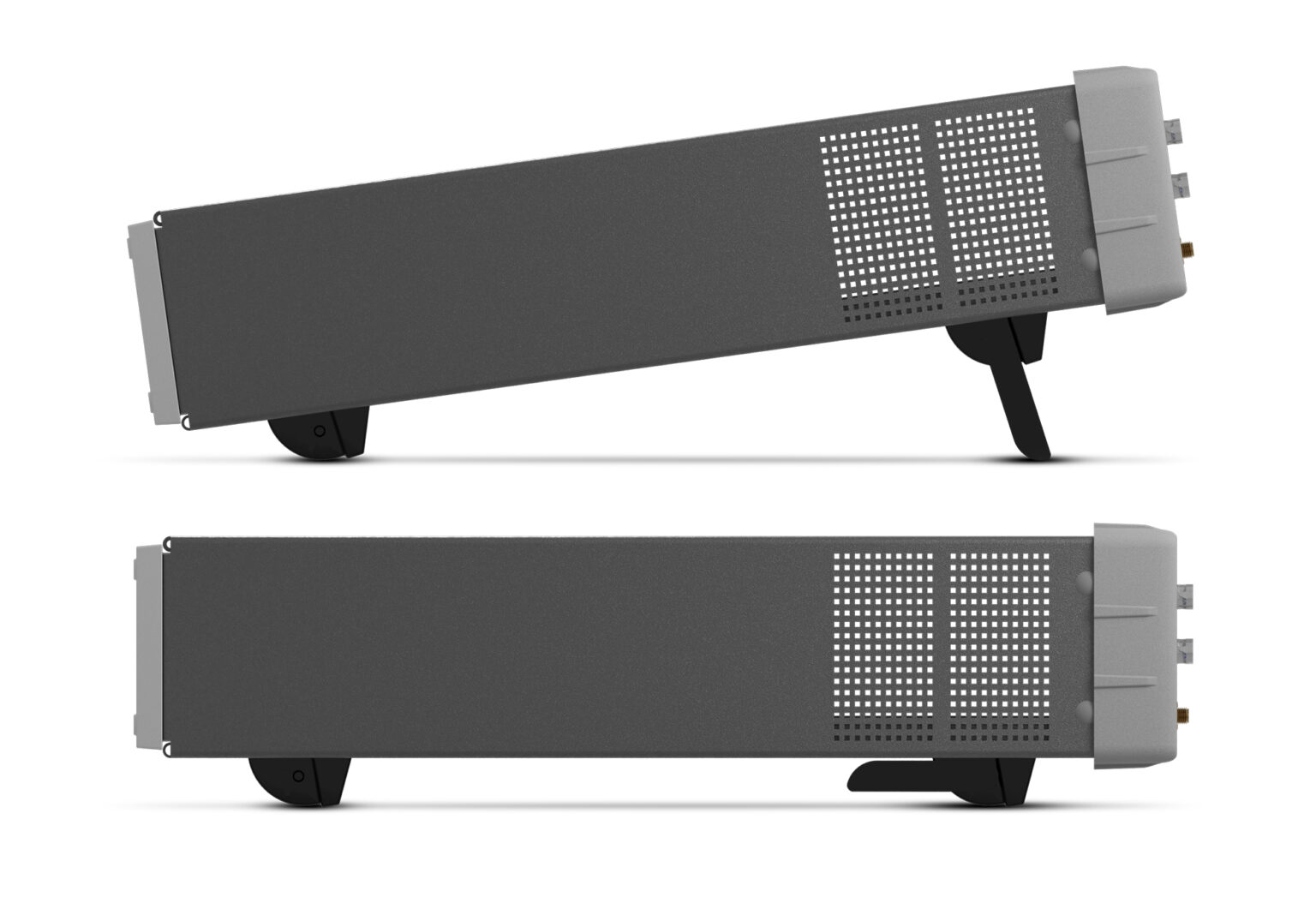
Fig. 1 Fold-down support for comfortable bench-top use.

Cleaning of the instrument

When cleaning the instrument, wipe it with a silicone cloth or soft cloth to remove dust or dirt. When it is hard to remove the dirt, wipe it with a cloth wet with water and dry the instrument completely after cleaning.

CAUTION :Never use any organic solvent such as benzene, acetone, etc.

Rackmount Adapter - one unit

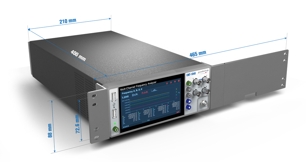
Fig. 2 Dimensions for rackmounting hardware.

If you have ordered a 19-inch rack-mount kit for your instrument, Option 22/90 for one instrument, it has to be assembled after delivery of the instrument. The rackmount kit consists of the following:

• 2 brackets, (short, left; long, right)

• 4 screws, M5 x 8

• 4 screws, M6 x 8

Warning

Do not perform any internal service or adjustment of this instrument unless you are qualified to do so.

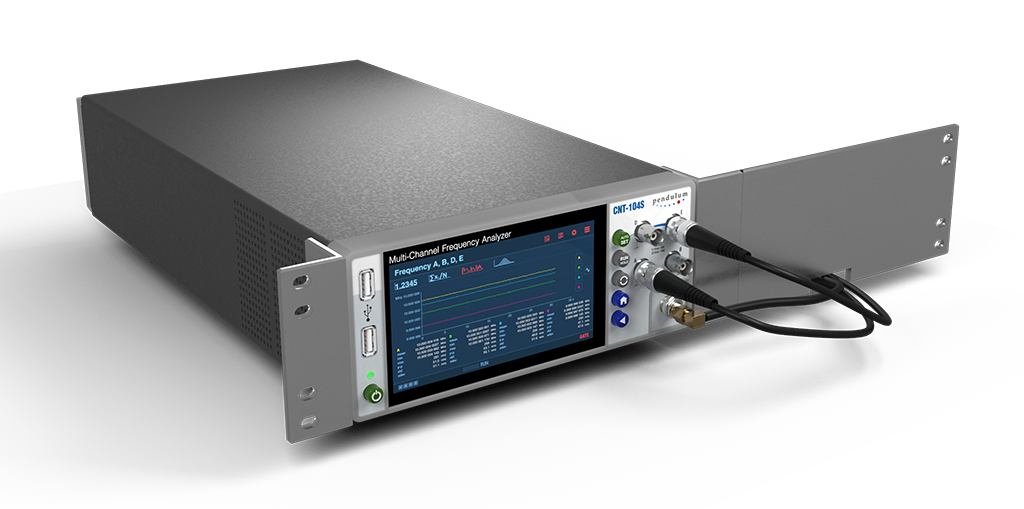
Fig. 3 Fitting the rack mount brackets on the instrument.

Assembling the Rackmount Kit (Option 22/90)

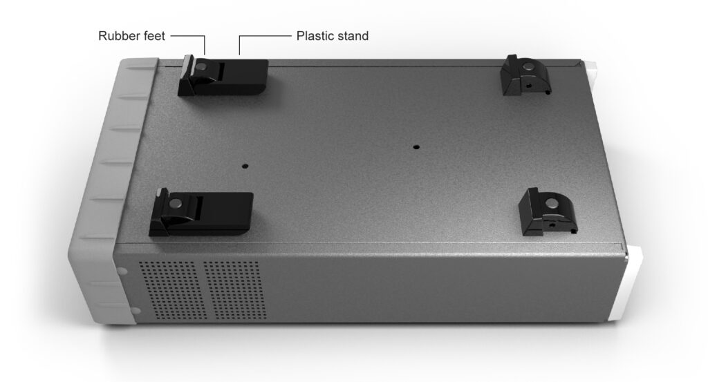
Fig. 4 Assembling the Rackmount Kit (Option 22/90)

• Turn the device upside down

• Remove the rubber feet in the plastic stand

• Loosen the screws underneath the rubber feet

• Remove the plastic stands

• Remove the rubber bumper around the front

• Remove the four decorative plugs that cover the screw holes on the right and left side of the front panel.

• The long bracket in Option 22/90 has an opening so that cables for Input signals can be routed inside the rack.

• Mount the rackmount kit with the included screws

Reversing the Rackmount Kit

The instrument may also be mounted to the right in the rack. To do so, swap the position of the two brackets.

Rackmount Adapter - two units

This rackmount adapter can hold any two standard Pendulum ½ x 19” units.

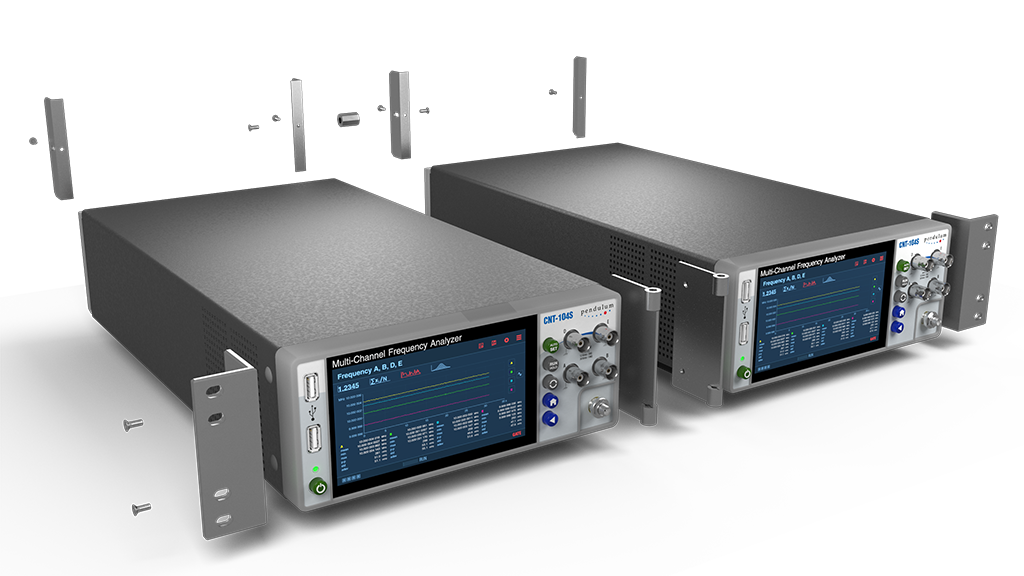
Fig. 5 Rackmount Adapter - two units

If you have ordered the Option 22/05 rack-mount kit for two instruments, it has to be also assembled after delivery of the instrument. The rackmount kit consists of the following:

• 4 Brackets, rear

• 1 Hinge Spring Latch

• 2 Ear, rack

• 1 Assembly instruction, SXS Rack kit

• 2 Screws M4x8

• 8 Screws M5x10

• 1 Spacer M4x16

Assembling the Rackmount Kit (Option 22/05)

Fig. 6 Assembling the Rackmount Kit (Option 22/05)

• Turn the devices upside down

• Remove the rubber feet in the plastic stand

• Loosen the screws underneath the rubber feet

• Remove the plastic stands

• Remove the rubber bumper around the front

• Remove the four decorative plugs that cover the screw holes on the right and left side of the front panel.

Use the following steps to complete the side by side rack mount installation for your products. If necessary, refer to the item numbers in the following diagram for additional detail.

• Determine where you would like each unit positioned (i.e., on the right or left side)

• If plugs exist on the mounting holes on the front left and right side of product cover, remove and discard them

• Using screwdriver, screw the rack ear (Item #2) into place using the supplied 10mm screws (Item #5)

• Pinch the hinge pins together to separate the right and left hinge halves (Items #3 and 4)

• Attach hinge halves to the unit with hinge facing towards the front (as displayed in diagram)

• Using a screwdriver, remove the existing rear brackets on the back of each unit

• Using existing machine screws removed in previous steps, attach the rear brackets supplied with the mounting kit (Item #1)

• Pinch the hinge pins together into the stored position. Align the hinge halves together between the two units, and swing together side by side. The hinge pins should snap into place securing the front of the two units together

• Take the supplied Hex Spacer (Item #7) and place between middle rear brackets, and secure using the supplied 8mm screws (Item #6)

• Assembly is now ready for installation into standard 19” rack

Fig. 7 Rackmount Adapter - two units

Getting Familiar with the Instrument

Front & Rear Panels

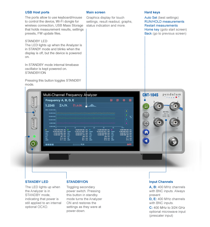
Fig. 8 Front panel of CNT-104S

Fig. 9 Rear panel of CNT-104S

Fig. 10 Rear panel of CNT-102

Home Screen

Note

Pictures below illustrate display of CNT-104S model.

For CNT-102, channels D, E are not available and areas, fields and graphical objects for corresponding to these channel are not present. Up to 2 signals can be measured in parallel.

For FTR-210R, channels B, D, E, C are not available and areas, fields and graphical objects for corresponding to these channel are not present. Only one signal can be measured in parallel.

Fig. 11 Numeric screen of CNT-104S

Measurement State:

• RUN – next measurement will start automatically as soon as current one is over. Pressing RESTART in this state starts new measurement, measurement state remains RUN. Pressing RUN/HOLD in this state changes the state to SINGLE, but current measurement continues. Exception is Totalize measurement functions, when state is changed to HOLD.

• SINGLE – measurement is in progress. After measurement is over – measurement state will change to HOLD, no new measurement will start. Pressing RESTART in this mode starts new measurement, measurement state remains SINGLE. Pressing RUN/HOLD in this state stops the measurement and changes state to HOLD.

• HOLD – measurement is not active. Results of previous measurement are displayed. Pressing RESTART starts new measurement and changes state to SINGLE. Pressing RUN/HOLD in this state starts new measurement and changes state to RUN.

Indicators:

• Trigger indicators – if signal crosses set trigger level(s) for particular input, then corresponding trigger indicator is lit, otherwise it is grayed out.

• GATE – red when measurement is active, grayed out otherwise.

• MATH – Math function is active. User selectable formula is applied to one or all (depending on user choice) measurement series.

• LIM – Limits function is active. Values of one or all (depending on user choice) measurement series are checked against the limit(s) specified by the user. User can configure the desired behavior when measurement data exceeds the limit(s).

• ER – External Reference clock is used as a timebase for measurements.

• REM – instrument is now in Remote state (controlled by remote application). In this state the instrument can not be controlled from the front panel. Press BACK to switch to Local state and enable front panel control. If REM! indicator is displayed, Remote Lockout mode is active and BACK button cannot be used to return to Local Mode. Only remote party can undo this state. In web interface or VNC client use F7 key in place of BACK.

• ARM – measurement configured to start and/or stop on arming signal.

Settings

Note

Pictures below illustrate display of CNT-104S model.

For CNT-102, channels D, E are not available and areas, fields and graphical objects for corresponding to these channel are not present. Up to 2 signals can be measured in parallel.

For FTR-210R, channels B, D, E, C are not available and areas, fields and graphical objects for corresponding to these channel are not present. Only one signal can be measured in parallel.

Fig. 12 Settings menu

Fig. 13 Arming menu

Fig. 14 Function and inputs selection menu

Inputs description:

• A, B, D, E – main inputs. Note, inputs D and E available only on four-channel models.

• A2, B2, D2, E2 – supplementary comparators of main inputs (e.g. for measuring time intervals inside multi-level signals). Note, D2 and E2 are available only on four-channels models.

• C – optional high frequency input

• EA – External Arming input

• ER – External Reference Input

Fig. 15 Numeric keyboard

Measurement Data Display

Note

Pictures below illustrate display of CNT-104S model.

For CNT-102, channels D, E are not available and areas, fields and graphical objects for corresponding to these channel are not present. Up to 2 signals can be measured in parallel.

For FTR-210R, channels B, D, E, C are not available and areas, fields and graphical objects for corresponding to these channel are not present. Only one signal can be measured in parallel.

View large numeric data from 4 measurement channels at the same time along with auxiliary data (e.g. voltage):

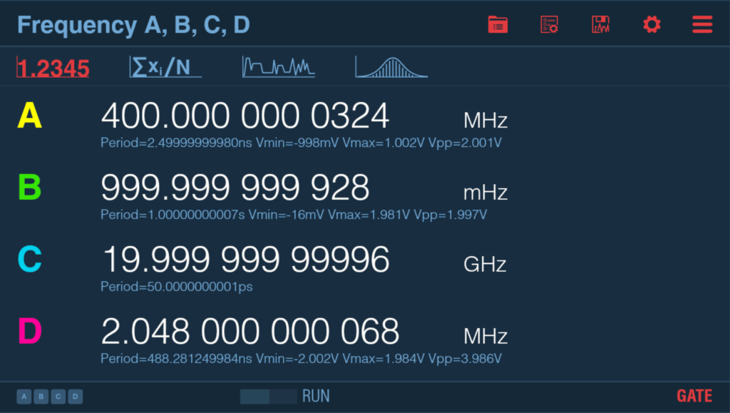
Fig. 16 Numeric screen

View detailed statistics for all measurement channels (click numbers for particular channel to zoom):

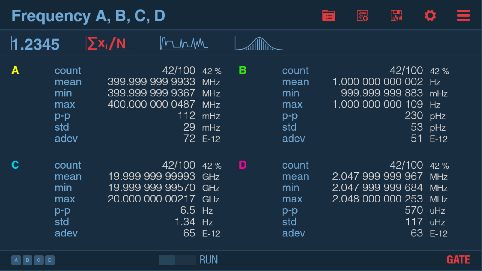
Fig. 17 Statistics screen

Fig. 18 Graphs screen

Fig. 19 Distrubution graph screen

Measurement principles and concepts

Time and Frequency measurement principles

Block diagram on Fig. 20 demonstrates input signal transformation to series of time and frequency measurement data points.

First, input signal gets into input amplifier. The generic role of input amplifier circuits is matching the input to signal source, and optionally: attenuate or amplify it, remove DC offset and/or filter out high-frequency noise.

Please note: There are several kinds of input amplifier circuits (configurable input amplifiers, prescalers, fixed input amplifiers), please refer to 4.5 Input signal conditioning/Input Amplifiers chapter for more details about them.

After the input amplifiers the signal is digitized using one (inputs C, EA, ER) or 2 comparators (inputs A, B, D, E on four-channel models, inputs A, B on two-channel models). It works the following way: when the signal crosses the set trigger level, comparator generates a positive (in case of transition from below to above the trigger level) or negative (in case of transition from above to below the trigger level) slope. Please refer to Fig. 21 for an example.

Please note: For most measurement modes on inputs with 2 comparators, output of only one comparator is used for measuring the signal from this input. However, there are measurement modes using both comparators implicitly:

• Rise/ Fall Time and Slew Rate measurements use 2 comparators for getting Time Interval between lowest (10%) and highest (90%) levels of the signal (see details in Rise Time, Fall Time, Rise-Fall Time);

• Pulse width and Duty Cycle measurements use 2 comparators to produce pulses on positive and negative slope of a signal and measure Time Interval between these;

• Frequency and Period Average use 2 comparators to implement implicit wide hysteresis targeted on improving noisy signals measurements (see details in Frequency/Period Average measurements chapter).

Second comparator can also be explicitly selected for measurement. E.g., Time Interval A, A2 will measure time interval between signal level set by trigger level A and signal level set by trigger level A2 (can be useful for measuring characteristics of multi-level signals, e.g. TDR measurements – see Measuring Time Interval between different trigger points of the same signal). It can also be explicitly used as a source of start or stop arming.

Digitized signals from physical inputs are just pulse trains which can be multiplexed to 4 internal measurement channels. Each measurement channel starts with Wide Hysteresis block. Wide Hysteresis block just passes through the signal for most measurement functions except Frequency, Period Average, their Smart versions, TIE, and Frequency Ratio for which implicit wide hysteresis is used for better noise tolerance (see Frequency/Period Average measurements).

The resulting pulse train is then counted independently in each measurement channel. Measurement logic specific for each measurement mode makes snapshots of channel’s pulse counter, timestamps it and adds channel number, forming series of so-called raw results.

Raw results are further post-processed in calculation block to form series of final value-timestamps pairs.

Note

Block diagram below illustrate logic of CNT-104S, CNT-104R.

For CNT-102, channel D, E circuits are not available.

For FTR-210R, channel B, D, E, C circuits are not available.

Fig. 20 Input signal to Time & Frequency measurement results transformation

Fig. 21 Example of input signal to result transformation for Frequency measurement mode with Wide Hysteresis

Voltage measurement principles

Measuring voltage of the input signal is available only on inputs A, B, D, E (for CNT-104S, CNT-104R) or on inputs A, B (for CNT-102) or on input A (for FTR-210R). On each input there are 2 comparators used to search for signal’s lower and upper levels. Multiple inputs can be measured in parallel.

Adaptive search algorithm is used which depends on Voltage Mode setting. Each voltage mode implies minimum input signal frequency which the voltage measurement can handle. E.g. in Normal Voltage mode (default) instrument is able to measure voltage of signals with frequencies starting with 100 Hz and above. Allowing lower frequencies makes the voltage measurement slower so it is not recommended to set Voltage mode below Normal unless really needed (one might want to consider using Autoset instead).

Table below summarizes Voltage Modes available :

Table 1 Voltage Modes

Voltage Mode	Minimum Frequency	Average Time to measure 1 voltage sample
Very Slow	1 Hz	15 s
Slow	10 Hz	1.5 s
Normal	100 Hz	450 ms
Fast	1 kHz	65 ms
Very Fast	10 kHz	30 ms

Sample Interval

On each measurement channel instrument can produce gap-free samples back-to-back as fast as 1 sample per 50 ns or 1 us (depending on particular model and licenses installed) which corresponds to setting Sample Interval to 0 s. However, for most cases one doesn’t need samples to be generated with such a high frequency, then using non-zero Sample Interval can be considered. In this case samples in each measurement channel will be generated not faster than once per set Sample Interval.

Fig. 22 Example of how sample interval works with 4-channels multi-channel Frequency measurement.

Sample Interval hints:

• Sample Interval clock is not synchronized to signal, meaning actual Sample Interval between 2 consecutive samples can be less or more than Sample Interval set by the user.

• When doing parallel measurement, sample interval is applied to each measured series independently. E.g., when measuring Frequency A, B, D, E and using 1 ms Sample Interval, one will get 1000 Frequency Samples per second from each input.

• Sample Interval for averaging measurement functions (Frequency, Period Average and their Smart alternatives) acts as an averaging gate. The larger the gate (Sample Interval) – the greater the resolution.

• The instrument contains two cascaded memories for result saving. The first is the cache buffer that can holdup to 20000 raw samples with a maximum writing speed of 20 million Samples/s. The second is the main memory, that can hold up to 32 million results, with a maximum writing speed of 12.5 million samples per second, or 80 ns between samples. The data is written to the cache buffer in parallel from up to 4 inputs, meaning the capture speed is independent of the number of inputs used. The data transfer from the fast cache buffer to the slower main memory is done in serial, so the maximum capture speed varies with the number of channels Setting max number of samples of samples to 20k for a single channel measurement, or 5k for a 4 channel measurement, will guarantee a sampling rate of 20 million values/s or 1 million values/s, at a sample interval of 50 ns or 1 us (depending on particular model and licenses installed). When setting a larger number of samples , the Sample Interval (given that signal period is less than or equal to the set Sample Interval) must be increased to minimum 80 ns for 1-channel and minimum 320 ns for 4-channel measurements, to avoid cache buffer overflow. If not, the measurement is aborted to avoid data loss.

Example. Measurement function is Frequency A,B,D,E, Sample Interval is |minimal_sample_interval|, Sample Count is set to 10000 and period of all input signals is 50 MHz. 4 measurement channels are used in parallel, each supposed to deliver samples at a rate of 20 million samples per second, which is greater than the speed cache buffer can be fetched with (12.5 million samples). Total number of samples to be generated is 4 x (10000 + 1) = 40004 (N + 1 raw samples are needed to calculate N frequencies), which is twice greater than measurement logic buffer capacity. So, the buffer will overflow and measurement will be aborted. Solution would be to either increase Sample Interval to 320 ns (4 channels x 80 ns, giving 12.5 million samples per second total) or to decrease Sample Count to 4999 (giving 4 x (4999 + 1) = 20000 samples total).

To avoid this situation please watch out for warning text when setting Sample Count and/or Sample Interval or warning icon when choosing measurement function and inputs.

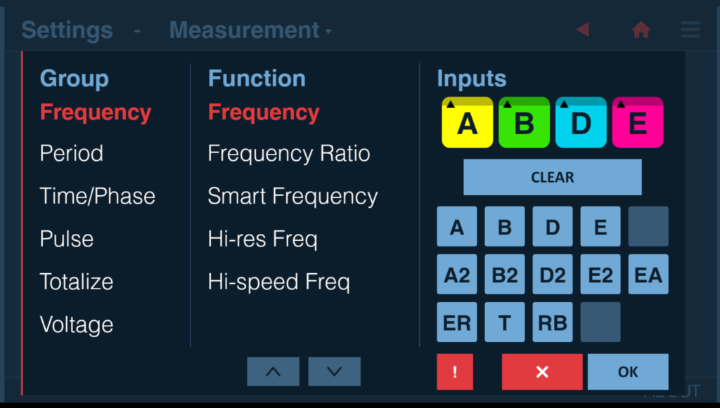
Fig. 23 Warning icon on Function/Inputs selection dialog ( clickable red button with exclamation sign to the left of Cancel).

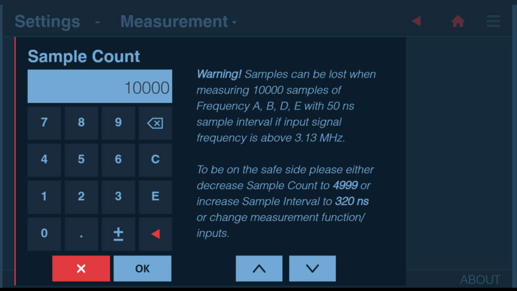
Fig. 24 Warning text when editing Sample Count

• When using Sample Interval close to 50 ns, actual sample interval might vary between 50 ns and 100 ns. In case of Time Interval measurement – it can result in generating less samples than was ordered by Sample Count setting. To avoid this please consider setting Sample Interval to 0 if you need minimal sample interval between samples. Setting Time Interval to 0 disables Sample Interval clock, meaning taking samples as fast as possible (close to 50 ns if signal period is 50 ns or greater).

  Note

  Above relates only to model and license combinations allowing sample interval of 50 ns.

• Sample Interval setting doesn’t affect Voltage measurement where interval between samples directly depends on Voltage Mode (please see Voltage measurement principles for details).

• Sample Interval setting doesn’t affect manual Totalize measurement where interval between samples is always 100 ms.

Input signal conditioning/Input Amplifiers

Overview

The input amplifiers are used for adapting the widely varying signals in the ambient world to the measuring logic of the instrument.

These amplifiers have many controls, and it is essential to understand how these controls work together and affect the signal.

Configurable amplifiers

Input amplifiers for inputs A, B, D, E (for CNT-104S, CNT-104R) or A, B (for CNT-102) or A (for FTR-210R) are configurable (Inputs page of the Settings dialog) and allow to select a bunch of parameters described in the following sections.

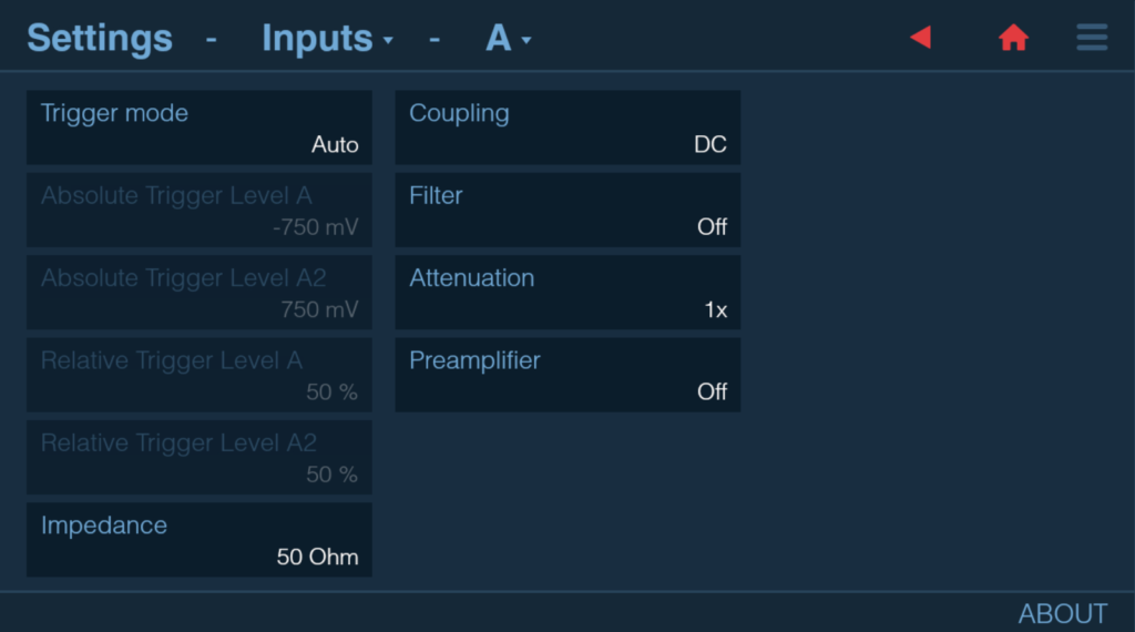
Fig. 25 Input amplifiers configuration menu

Impedance

Impedance setting allows to match the impedance of the input to signal source. One can choose between 1 MΩ or 50 Ω impedance.

CAUTION: Switching the impedance to 50 Ω when the input voltage is above 12 Vrms may cause permanent damage to the input circuitry.

Attenuation

This setting allows attenuating the signal by factor of 10 if its dynamic range exceeds ±5 V. 1x, 10x and AUTO attenuation options are available. If AUTO is selected then first sample of any voltage measurement (including the ones performed during Autoset and Auto-trigger) will be analyzed to determine the dynamic range of the signal. If the range exceeds ±5 V then 10x attenuation will be switched on automatically. 1x will be used otherwise.

Coupling

Use the AC coupling feature to eliminate unwanted DC signal components or keep DC offset by using DC coupling.

Hint: Always use AC coupling when the AC signal is superimposed on a DC voltage that is higher than the trigger level setting range. However, we recommend AC coupling in many other measurement situations as well. When you measure symmetrical signals, such as sine and square/triangle waves, AC coupling filters out all DC components. This means that a 0 V trigger level is always centered around the middle of the signal where triggering is most stable.

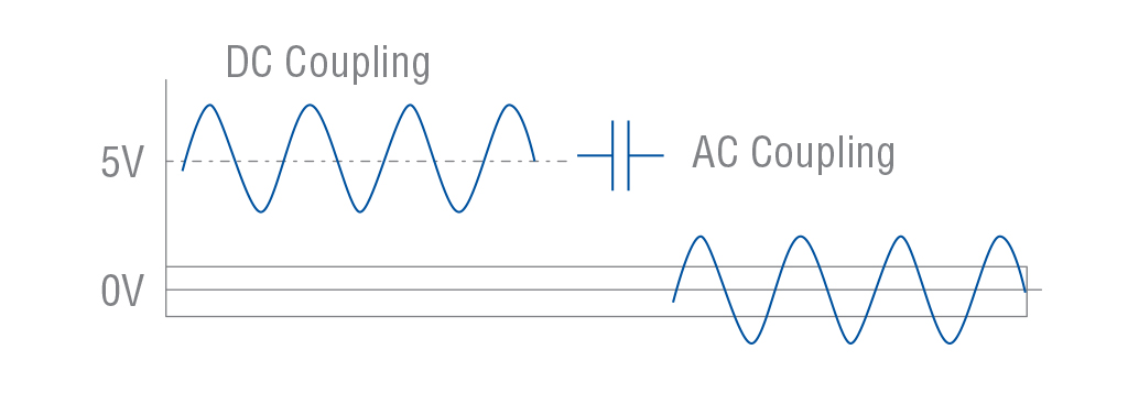
Fig. 26 AC coupling a symmetrical signal

Hint: Signals with changing duty cycle or with a very low or high duty cycle do require DC coupling. Fig. 27 shows how pulses can be missed, while Fig. 28 shows that triggering does not occur at all because the signal amplitude and the hysteresis band (please see for explanation of what is Hysteresis Band) are not centered.

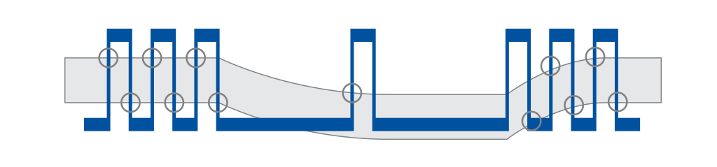
Fig. 27 Missing trigger events due to AC coupling of signal with varying duty cycle.

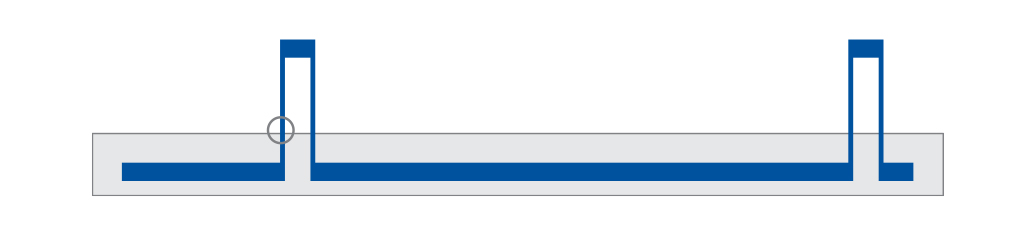
Fig. 28 No triggering due to AC coupling of signal with low duty cycle.

Hint

Always use DC coupling for signals below 10 Hz.

Filter

This setting allows you to apply analog low-pass filter for signals with high-frequency noise or interference. 10 kHz and 100 kHz low-pass filters are available. All filters have a signal rejection slope of approx. 20 dB / decade.

Hint: keep filters off unless you cannot obtain stable readings otherwise.

Hint: it is not recommended to use filters for pulse signals as filters affect pulse signal shape.

Preamplifier

Preamplifier allows to amplify the signal to improve sensitivity for signals with amplitudes below 100 mVpp.

Hint: avoid using pre-amplification if signal amplitude is above 100 mVpp. Prefer using Autoset instead – it will turn on pre-amplification only if necessary

Trigger Level

Set trigger level. Setting proper trigger level is essential for getting accurate and stable results. So it is advised to keep Trigger Mode Auto letting the instrument select adequate trigger levels. Please see Measurement Functions.

In Auto and Relative Trigger Modes, the instrument performs voltage measurement (using current Voltage Mode setting) – so-called auto-trigger – before each Time or Frequency measurement which delays the measurement start. In cases when it is undesirable, please use Manual Trigger Mode.

When measuring non-continuous signals or single cycles, auto-trigger might fail to measure signal voltage range correctly which won’t allow setting trigger levels properly and might result in wrong measurement results. It is advised to use Manual Trigger Mode in this case.

In Manual Trigger Mode in most cases one can get the best results if Trigger Level is set to the center of signal voltage range. It will help avoid capturing signal edge artifacts and in most cases the middle of the signal voltage range will be the point with maximum slew rate, which minimizes timing trigger error.

Setting trigger level close to signal minimum or maximum level can result in intermittent readings and/or unreliable result. For example, measured Frequency value twice greater or twice lower than actual can be a typical consequence of poor trigger level choice when measuring pulse signals with significant artifacts on edges.

Please note: Actual triggering does not occur when the input signal crosses the trigger level at 50 percent of the amplitude, but when the input signal has crossed the entire hysteresis band (Figure 11). Which causes measurement timing errors.

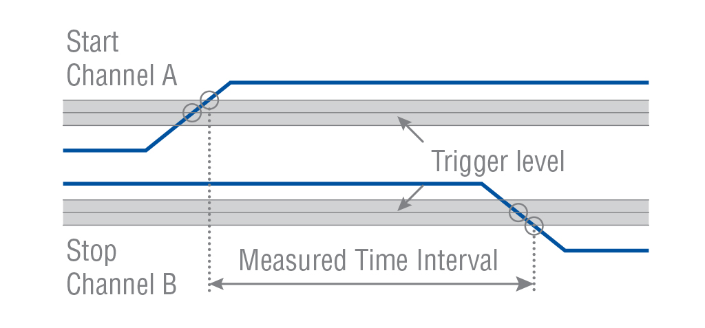
Fig. 29 Trigger hysteresis

The hysteresis band is about 20 mV with attenuation 1x, and 200 mV with attenuation 10x. The hysteresis compensation reduces hysteresis trigger error to <2 mV

To keep the hysteresis trigger error low, the attenuator setting should be 1x when possible. Use the 10x position only when input signals have excessively large amplitudes, or when you need to set trigger levels exceeding the -5 V to +5 V window.

Input Amplifiers with fixed configuration

The following inputs have fixed amplifier parameters:

• EA (External Arming) is fixed to 1 kΩ impedance and approx. 1.5 V trigger level;

• ER (External Reference) is fixed to 50 Ω impedance and accepts signals with 0.1 to 5 V_rms amplitude;

• C (Prescaler input) is fixed to 50 Ω impedance.

Arming

Arming, in general, gives the opportunity to start and stop a measurement when an external qualifier event occurs.

Arming can initialize either a single sample acquisition (Arm on Sample) or a single measurement session defined by sample count (Arm on Block). Measurement can be started and stopped by rising or falling edge of signals on instrument’s inputs and delayed from 0 ns (delay off) to 2 s with 10 ns resolution step. In case of Totalize measurement mode, timer (set by a combination of Sample Interval and Stop Source set to Timer) can be used as a source of stop arming.

Table 2 shows possible arming modes and their specifics. Modes absent in this table are not supported.

Table 2 Arming modes and their specifics

Start Arming Source	Stop Arming Source	Arm on	Measurement Function	Comment
Off	Off	N/A	Any	Arming is not used, measurement is started and stopped normally
Input	Off	Block	Any, except Totalize	Start arming input initialize measurement session (block). Measurement session ends when all samples (number is set by Sample Count) have been collected. 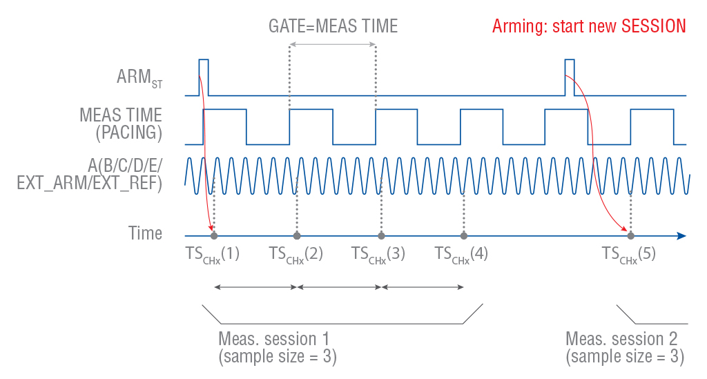Fig. 30 Frequency measurement with measurement session repeated after start arming pulses Arming start pulses that occur during measurement session are neglected. 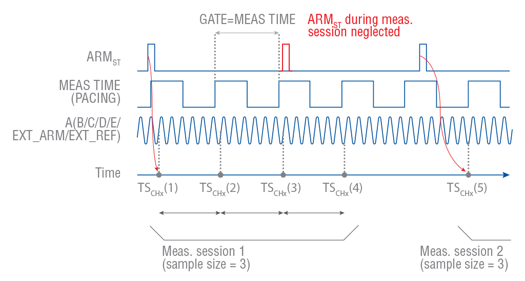Fig. 31 Frequency measurement with arming start pulses occurring during the measurement session
Input	Input	Block	Any, except Totalize	Start arming starts measurement session (block). Measurement session ends when either all samples (number is set by Sample Count) have been collected or by signal front on stop arming input (whatever comes first). 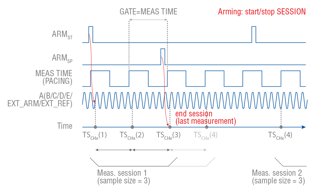Fig. 32 Frequency measurement with measurement session controlled by start and stop arming signals
Off	Timer	Sample	Totalize	Totalize measurement is started by pressing Restart button, Sample Interval defines Totalize Gate length. The Analyzer counts number of events during the gate and produces single sample (1 sample per series).
Input	Timer	Sample	Totalize	Start arming pulses start Totalize Gates (gate length is defined by Sample Interval). Each gate produces 1 sample (per series). Measurement session ends once required number of samples (set by Sample Count) was collected. 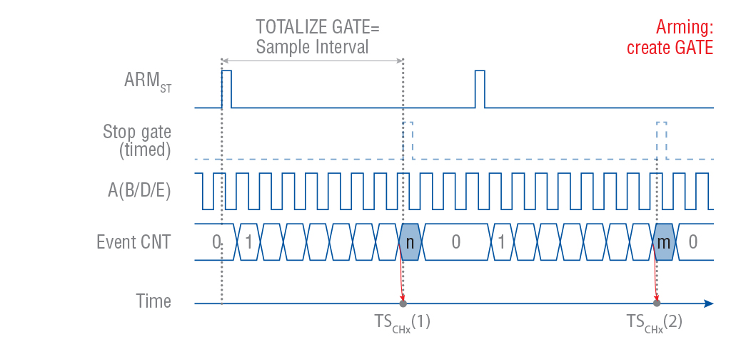Fig. 33 Totalize measurement in timed mode (stop arming signal set to timer)
Input	Off	Sample	Any, except Totalize	Start arming is used as a pacing clock – single sample measurement is executed just after the arming event. 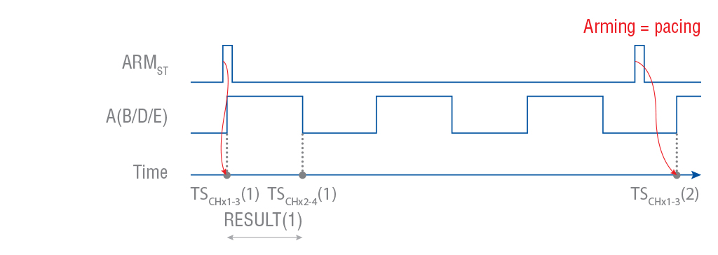Fig. 34 Pulse width measurement with arming signal used as a pacing clock In case of Frequency/Period Average measurement, samples are measured with dead-time, no back-to-back. Maximum total number of samples is reduced to up to 16 million. 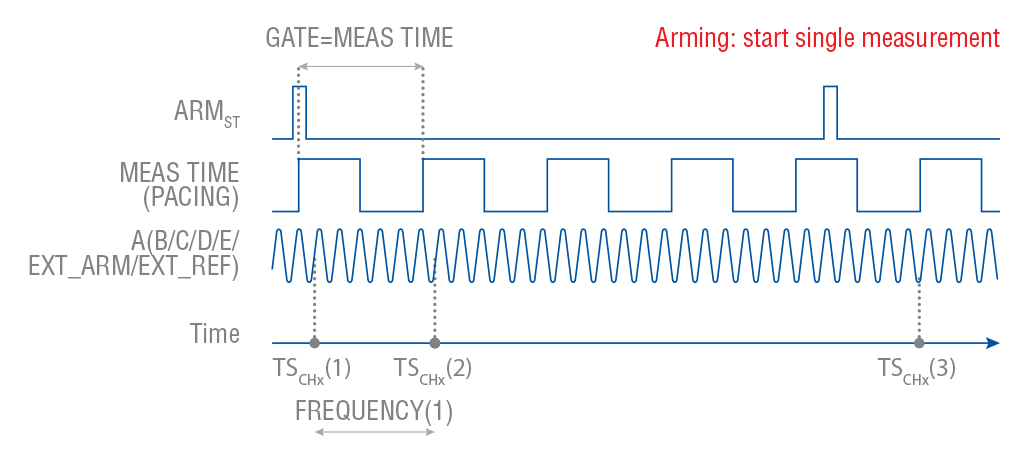Fig. 35 Frequency measurement initialized by arming pulses
Input	Input	Sample	Totalize, Frequency, Period Average, Smart Frequency, Smart Period Average	Start arming events start Gate (gate length is defined by Sample Interval). Stop arming events end Gate. Each gate produces 1 sample (per series). Measurement session ends once required number of samples (set by Sample Count) was collected. In case start and stop arming settings are not the same, neasurements are performed with dead-time, no back-to-back. Maximum total number of samples is reduced to up to 16 million. 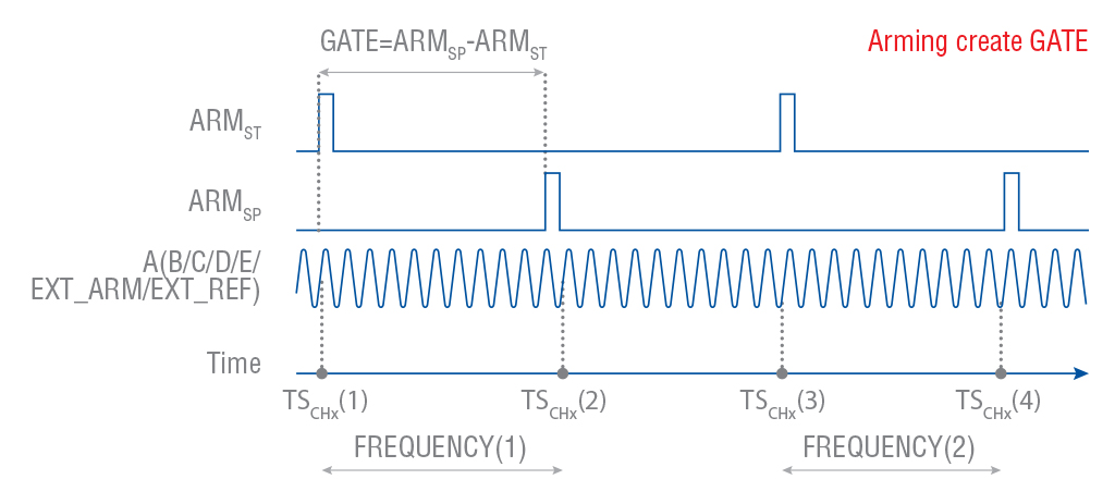Fig. 36 Frequency measurement in a gate created by arming signals When arming start and stop conditions are the same, measurements are performed continuously (back-to-back) with no dead-time. 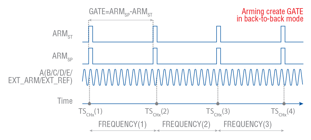Fig. 37 Frequency measurement when arming stop is set the same as arming start (back-to-back measurements) n case Smart versions of Frequency/Period Average are used, each sub-gate (Sample Interval divided by 1000) is being armed, i.e. one sample is calculated using data from 1000 arming gates.
Input	Input	Sample	Any, except Totalize, Frequency, Period Average, Smart Frequency, Smart Period Average	Start arming is used as a pacing clock – a single sample measurement is executed just after active edge of arming pulse. Stop arming delays registration of timestamps other than the first one.   Depending on particular measurement mode, two, three or four timestamps are registered that give a single result. 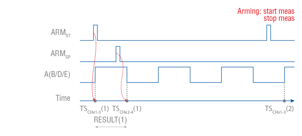Fig. 38 Pulse width measurement with arming on sample and start and stop arming active, case 1 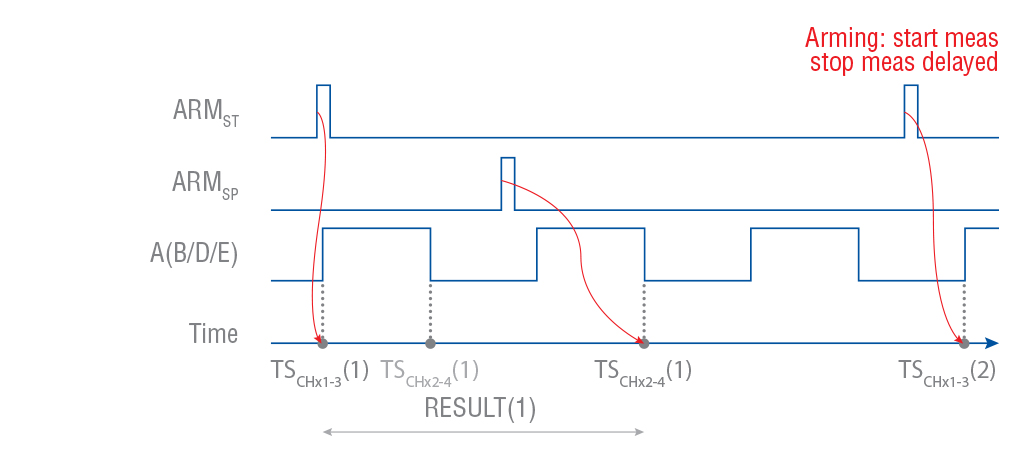Fig. 39 Pulse width measurement with arming on sample, start and stop arming active, case 2

Start arming is useful for measurement of frequency in signals, such as the following:

• Pulse modulated RF signals (bursts) Single-shot events or non-cyclic signals.

• Pulsed signals where pulse width or pulse positions can vary. Signals with frequency variations versus time (“profiling”).

• A selected part of a complex waveform signal.

Signal sources that generate complex wave forms like pulsed RF, or sweep signals, usually also produce a sync signal that coincides with the start of a sweep, or start of a radar burst. These sync signals can be used to arm the instrument. See Fig. 40.

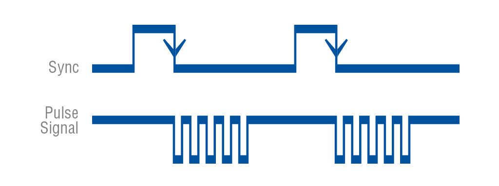
Fig. 40 Sync signal used as start arming starts the measurement.

You normally use stop arming together with start arming. That means that the external gating signal controls both the start and the stop of the measurement. Such a gating signal can be used to measure the frequency of an RF burst signal. Here the position of the external gate must be inside a burst. See Fig. 41.

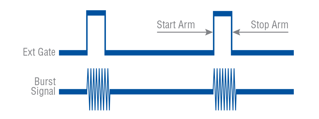
Fig. 41 Start and stop arming together is used for burst signal gating.

Note that burst measurements with access to an external sync signal are performed in the normal Frequency mode. In time interval measurements, you can use the stop arming signal as a sort of “external trigger Hold Off signal”, blocking stop trigger during the external period. See Fig. 42.

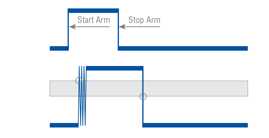
Fig. 42 Using start/stop arming as an external Hold-Off

Please note: start arming setup time is up to 5 ns. Which means that the measurement is actually started within 5 ns since start arming event.

Measurement Functions

Note

Particular measurement function availability depends on particular model and licenses combination.

Frequency/Period

There are several functions suited for measuring Frequency or Period. Next sections provide details about each particular function and when one should be preferred over another.

Frequency/Period Average measurements

These are the most universal measurement functions for Frequency and Period. In this mode each sample is a Frequency/Period value averaged over sample interval (which acts as gate).

This is back-to-back measurement with no dead-time between the samples (see chapter Arming for exceptions). Multiple input signals can be measured in parallel. Minimal sample interval is 50 ns or 1 us (depending on particular model and licenses installed). Up to 32 million samples total can be measured in a single measurement session. Resolution is 12 digits per 1 s of gate time (Sample Interval).

If the signal period is greater or equal to the set Sample Interval – each signal period can be captured. When measuring Frequency/Period Average on inputs A, B, D, E and Trigger Mode is set to Auto or Relative, wide hysteresis (see details below) is used to improve noise tolerance. In this mode 2 comparators with different trigger levels are used for each input. First trigger level (e.g. Trigger Level A) defines the upper limit of wide hysteresis band and the second one (e.g. Trigger Level A2) defines the lower limit. Trigger Mode Auto sets trigger levels to 60% and 40% of signal’s voltage range and Relative allows modifying them to fine tune the hysteresis band.

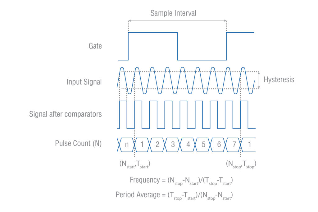
Fig. 43 Frequency/Period Average measurement with Wide Hysteresis

Without wide hysteresis, the signal needs to cross the approx. 20 mV in case of 1x Attenuation (200 mV in case of 10x) input hysteresis band before triggering occurs. This hysteresis prevents the input from self-oscillating and reduces its sensitivity to noise. If signal noise is comparable or higher than hysteresis band – it can result in false extra triggering producing erroneous counts. These could ruin the measurement.

Fig. 44 shows how spurious signals can cause the input signal to cross the trigger or hysteresis window more than once per input cycle and give erroneous counts. Fig. 45 shows that a wide enough hysteresis prevents false counts.

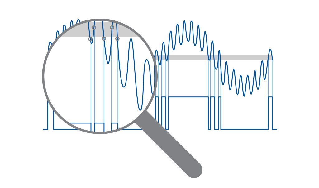
Fig. 44 Too narrow hysteresis gives erroneous triggering on noisy signals.

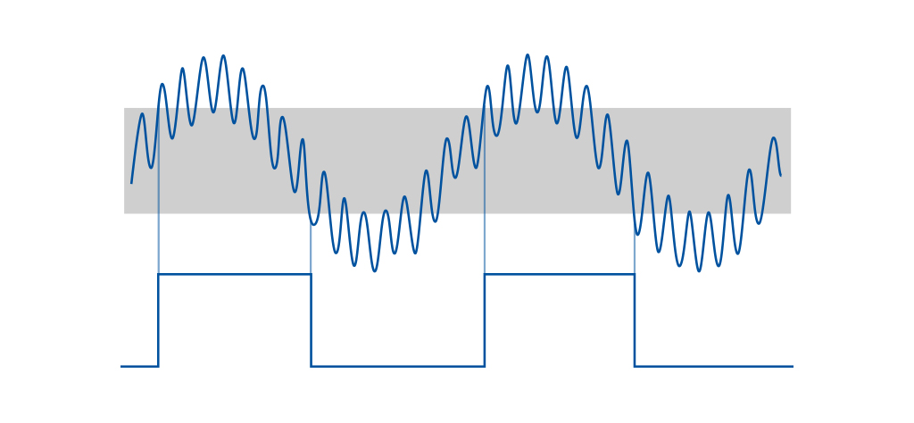
Fig. 45 Wide trigger hysteresis gives correct triggering.

Frequency C measurement.

With an optional RF input prescaler the instrument can measure up to 3, 10, 15, 20, or 24 GHz on Input C. These RF inputs are fully automatic, and no trigger setup is required. Set Sample Interval to achieve optimal compromise between resolution (long Sample Interval) and speed (short Sample Interval). The optional RF input C contains a prescaler that divides the RF signal with an integer value (Prescaler factor), to enable the normal counting circuitry to measure the frequency. The Option 10 (3 GHz) divides by 16, and the option 110/xx (10 to 24 GHz) divides by 64.

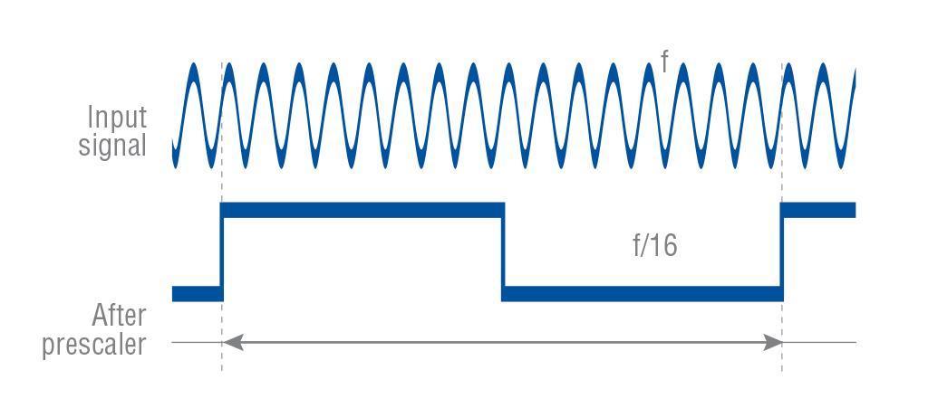
Fig. 46 Divide-by-16 Prescaler.

Fig. 46 shows the effect of the 3 GHz prescaler. For each 16 input cycles, the prescaler gives one square wave output cycle. An input frequency of let’s say 1.6 GHz is divided down to 100 MHz and measured by the normal counting circuitry. The display shows the correct input frequency since the microcomputer compensates for the effect of the division factor.

Prescalers do not reduce resolution. The relative quantization error is the same: 12-13 digits for 1s Sample Interval (Gate Time). See Table 3 to find the prescaler factors.

Table 3 Prescaler factors

Function	Prescaling Factor
All functions on inputs A, B, D, E (CNT-104S, CNT-104R) or A, B (CNT-102), also EA, ER	1
Frequency C (option 10: 3 GHz)	16
Frequency C (option 110: 10, 15, 20 or 24 GHz)	64

Smart Frequency/Period

Smart Frequency/Period is based on the same principle as normal Frequency/Period Average. Measurement gate is divided into 1000 sub-gates, giving additional samples and statistics resolution enhancement algorithm is applied on top of it. Thanks to that it allows to get up to 1 extra digit of resolution per 1 s of gate time (depending on input signal and measurement settings).

This comes with expense of additional constraints though. Minimal possible Sample Interval for Smart Frequency/Period is 50 us or 1 ms (depending on particular model and licenses installed). With Sample Interval less than 40 ms it is possible to measure up to 32000 samples per measurement session. Setting Sample Interval to 40 ms or more allows to get up to 4290000 samples per measurement session.

This is back-to-back measurement with no dead-time between the samples (see chapter Arming for exceptions). Multiple signals can be measured in parallel. Wide Hysteresis is used in Trigger Modes Auto and Relative.

Smart Frequency/Period is the best choice when one needs maximal possible resolution and can bear with lower sampling rate and sample count per session.

Please, note: resolution enhancement algorithm is based on the assumption that signal frequency is static. If it is not the case – the algorithm won’t be effective and it might make sense to fall back to normal Frequency/Period Average. Please note: section Frequency C measurement. Applies to Smart Frequency C as well.

Period Single

This measurement function is handy if one needs to capture individual periods of continuous signals or single cycles which are less than 50 ns. Individual periods starting from 2.5 ns can be captured.

This is not a back-to-back measurement, meaning that there is a dead-time of 50 ns or 1 us (depending on particular model and licenses installed). Up to 2 signals can be measured in parallel (depending on particular model). Up to 16 million samples total can be measured in a single measurement session.

Unlike Frequency/Period Average and their Smart versions, Period Single doesn’t use wide hysteresis. So only one comparator is used on A, B, D, E (CNT-104S, CNT-104R) or on A, B (CNT-102) and Trigger Mode Auto sets trigger level to the middle of signal voltage range (Relative Trigger Level 50%).

Please, note: when measuring non-continuous signal or single cycles, Trigger Mode Auto/Relative might fail to find proper trigger level. One need to fall back to Manual Trigger Mode in this case.

Frequency Ratio

In Frequency Ratio mode, the instrument measures Frequency Average of up to 4 signals in parallel (depending on particular model and settings) and then divides the resulting frequencies.

This is back-to-back measurement with no dead-time between the samples. 4 input signals can be measured in parallel for CNT-104S, CNT-104R, 2 - for CNT-102. Minimal sample interval is 50 ns or 1 us (depending on particular model and licenses installed). Up to 16 million samples total can be measured in a single measurement session.

Time Interval and Phase

Time Interval

This function allows to measure phase delay between clock signals with the same nominal frequency. At least N + 1 signal cycles are needed on each measurement input to get N Time Interval samples.

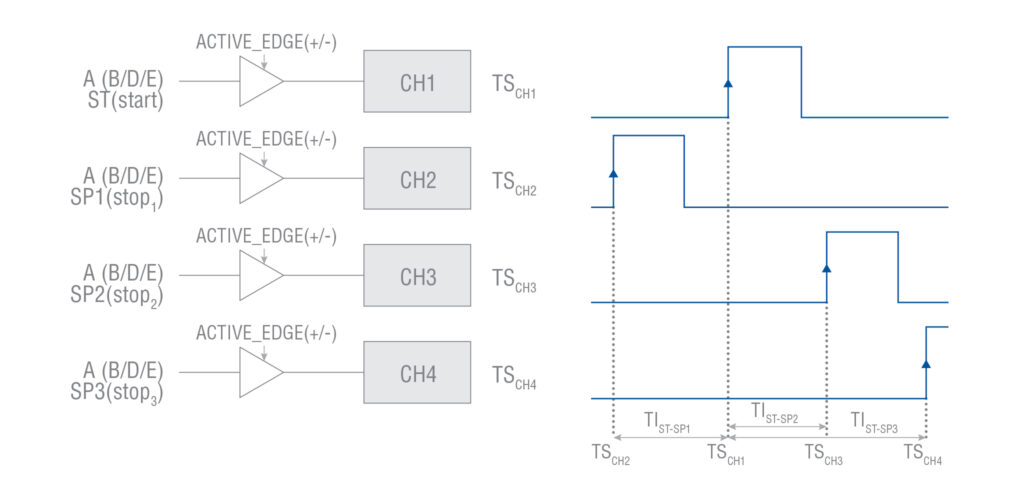
Fig. 47 Time Interval Continuous measurement mode

Time intervals in the range [-1000 s .. 1000 s] can be measured. Resulting values are normalized to always be in the range [-0.5 * Period .. Period].

4 input signals can be measured in parallel for CNT-104S, CNT-104R, 2 - for CNT-102. Minimal sample interval is 50 ns or 1 us (depending on particular model and licenses installed). Up to 16 million samples total can be measured in a single measurement session.

Please note: Time Interval Continuous is not suitable for measuring time interval between single shot events, use Time Interval Single instead.

When using Sample Interval close to 50 ns, actual sample interval might vary between 50 ns and 100 ns. In case of Time Interval measurement – it can result in generating less samples than was ordered by Sample Count setting. To avoid this please consider setting Sample Interval to 0 if you need minimal sample interval between samples. Setting Time Interval to 0 disables Sample Interval clock, meaning taking samples as fast as possible (close to 50 ns if signal period is 50 ns or greater).

Note

Above relates only to model and license combinations allowing sample interval of 50 ns.

Accumulated Time Interval

Accumulated Time Interval is useful for comparing phase delay between signals with the same nominal frequencies, but when frequencies of individual signals have small constant offset to each other. Time Interval will gradually increase over time and then drop after reaching value equal to signal Period, thus forming a sawtooth like graph. Accumulated Time Interval corrects this by adding or subtracting signal Period to Time Interval values when necessary. Other than that, it is exactly the same measurement as Time Interval Continuous.

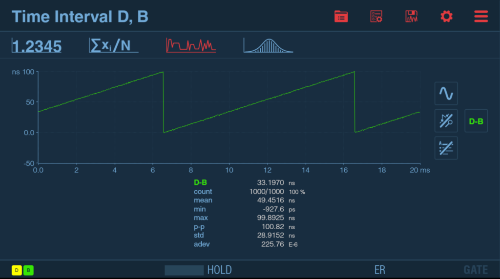
Fig. 48 Time Interval Continuous of 2 clock signals with constant frequency offset

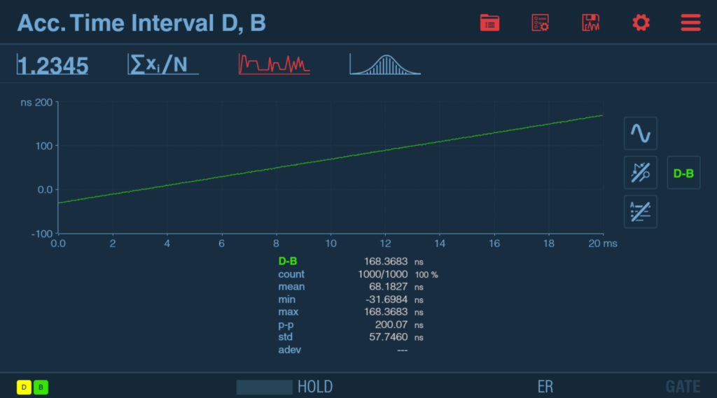
Fig. 49 Accumulated Time Interval of the same clock signals

As can be seen on Fig. 48 and Fig. 49, Accumulated Time Interval gives much better view on relative clock drift over time.

Time Interval Single

This function should be used to measure Time Interval between single events. Sample Interval setting is discarded, samples are captured as fast as it is possible.

Time intervals in the range [-1000 s .. 1000 s] can be measured. Resulting values are not normalized.

4 input signals can be measured in parallel for CNT-104S, CNT-104R, 2 - for CNT-102. Minimal sample interval is 50 ns or 1 us (depending on particular model and licenses installed). Up to 16 million samples total can be measured in a single measurement session.

Measuring Time Interval between different trigger points of the same signal

Thanks to the presence of two comparators on each of A, B, D, E (CNT-104S, CNT-104R) or A, B (CNT-102) inputs it is possible to measure Time Interval, Accumulated Time Interval, Time Interval Single, Phase and Accumulated Phase between two trigger points inside the same signal.

This can be useful for measuring intervals inside multi-level a signal, e.g. TDR measurement.

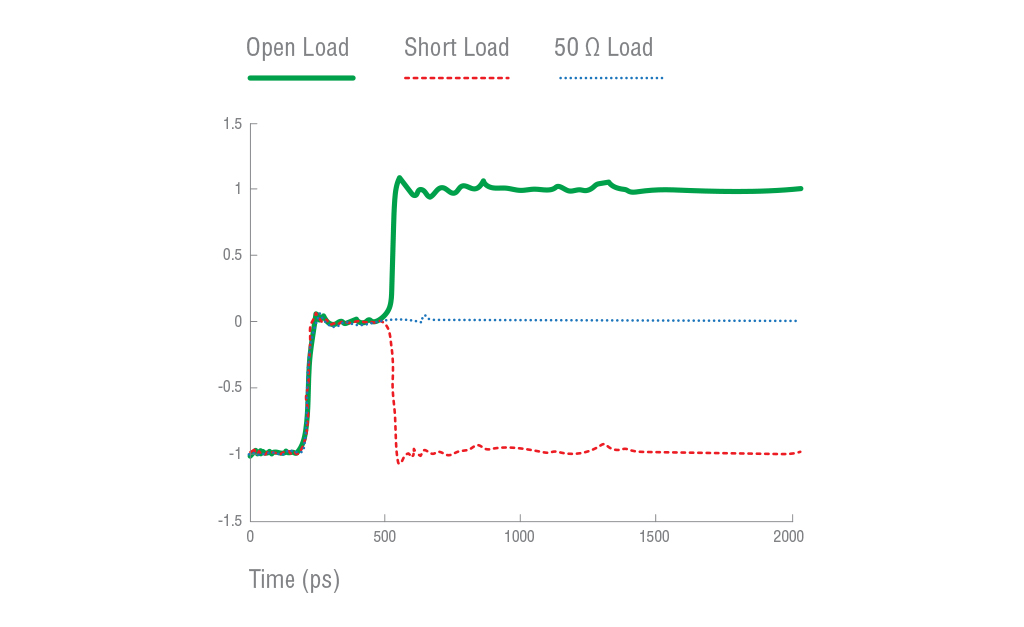
Fig. 50 Measuring Time Interval between 2 levels of reflected signal in TDR measurement allows to calculate the distance to cable break

Note

Pictures below illustrate display of CNT-104S model.

For CNT-102, channels D, E are not available and areas, fields and graphical objects for corresponding to these channel are not present. Up to 2 signals can be measured in parallel.

For FTR-210R, channels B, D, E, C are not available and areas, fields and graphical objects for corresponding to these channel are not present. Only one signal can be measured in parallel.

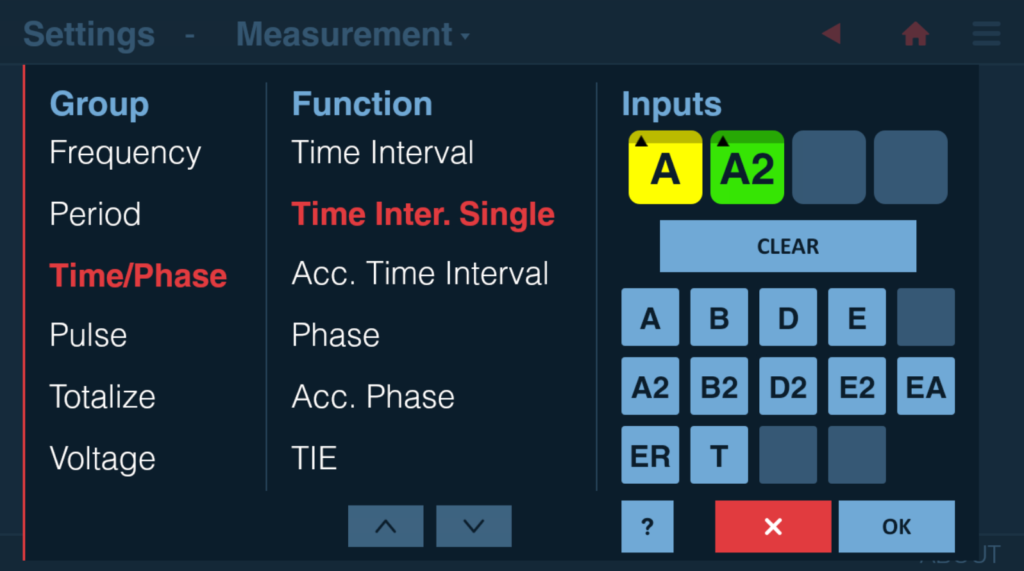
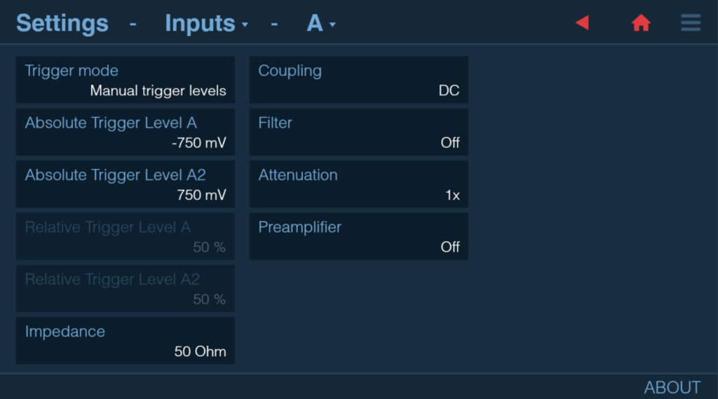
Fig. 51 Instrument’s configuration for TDR measurement on Figure 28

Another example is measuring time interval from start on input A positive slope to input A negative slope to input B positive slope to input B negative slope. This can be achieved by selecting Time Interval A, A2, B, B2 and specifying trigger levels and slopes accordingly (see Fig. 52).

Fig. 52 Time interval A-A2-B-B2 function selection

Fig. 53 Example configuration for Time Interval A to A to B to B measurement

Fig. 54 Example configuration for Time Interval A to A to B to B measurement

However, Time Interval A to A to A to A is not possible since that would require 4 different trigger conditions on input channel A, while only 2 comparators are present.

Phase

Phase is similar to Time Interval but with phase delay expressed as angle. This measurement assumes same nominal frequency on all measured inputs. At least N + 1 signal cycles are needed on each measurement input to get N Phase samples.

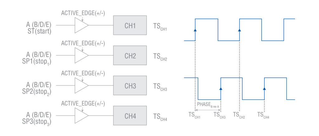
Fig. 55 Phase measurement mode

During this measurement, the instrument estimates continuous Time Interval and clock Period and calculates Phase as following:

Phase= 360°×((Time Interval)/Period)

where

Time Interval=TS_CH3-TS_CH1Period= TS_CH2-TS_CH1

Resulting Phase values are normalized to always be in the range [-180° .. 360°].

2 input signals can be measured in parallel for CNT-104S, CNT-104R, 1 - for CNT-102.. Minimal sample interval is 50 ns or 1 us (depending on particular model and licenses installed). Up to 16 million samples total can be measured in a single measurement session.

The typical measurement case is to measure the phase shift in various electronic components or systems, for example, filters or amplifiers. In this case, the input A signal is the input signal to the filter/amplifier, and the input B signal is the output signal from the filter/amplifier. That means that the input A and B signals are typically sine waves, with exactly the same frequency per test point, and the phase should be constant with zero drift (per test point).

Another typical use case is to compare two ultra-stable signals from different sources, but with the same nominal frequency, and express their phase difference in degrees. Then the signal shape could be both sine or pulse, and there is a possibility for a small phase drift between the signals.

Accumulated Phase

The same as for Time Interval, there is an Accumulated version of Phase measurement function to ease drift visualization over time when clock signals in comparison have same nominal frequency with a slow phase drift. But it has no meaning for phase measurements on sources with a more erratic behavior, or when the two frequencies are not the same.

Time Interval Error (TIE)

Please note: license is needed to unlock TIE option.

TIE measurement uses continuous back-to-back time-stamping to observe slow phase shifts (wander) in nominally stable signals during extended periods of time. The measurement itself is performed the same way as Frequency/Period Average but different processing is applied.

TIE is only applicable to clock signals, not data signals. Monitoring distributed PLL clocks in synchronous data transmission systems is a typical application.

The nominal frequency of the signal under test can be either manually or automatically set. Auto detects the frequency from the first samples, and rounds to number of digits set by the user (5 by default). TIE is measured as the period deviation of the input signal from the “ideal” reference period, and the accumulated deviation, up or down, is calculated for each Sample Interval, and displayed.

4 input signals can be measured in parallel for CNT-104S, CNT-104R, 2 - for CNT-102. Minimal sample interval is 50 ns or 1 us (depending on particular model and licenses installed). Up to 32 million samples total can be measured in a single measurement session. Resolution is 12 digits per 1 s of gate time (Sample Interval).

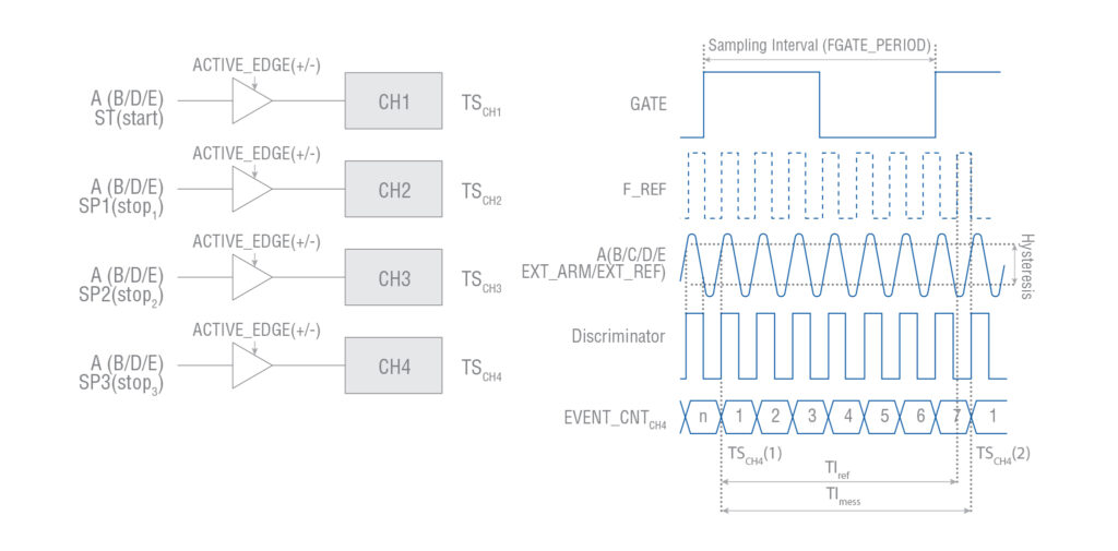
Fig. 56 TIE measurement

TIEA_(B/D/E)(i) = TS_CHx (i)-TS_CHx (1)-(((EVENT_CNT_CHx (i)-EVENT_CNT_CHx (1))/F_ref)

Pulse characterization

Positive and Negative Pulse Width

Positive pulse width measures the time between a rising edge and the next falling edge of the signal. Negative pulse width measures the time between a falling edge and the next rising edge of the signal.

The selected trigger slope is the start trigger slope. The instrument automatically selects the inverse polarity as stop slope.

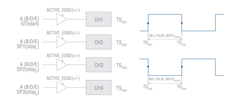
Fig. 57 Pulse width measurement

This is not a back-to-back measurement, meaning that there is a dead-time of 50 ns or 1 us (depending on particular model and licenses installed) between the samples. 2 input signals can be measured in parallel for CNT-104S, CNT-104R, 1 - for CNT-102.. Up to 16 million samples total can be measured in a single measurement session.

Positive and Negative Duty Cycle

Duty cycle (or duty factor) is the ratio between pulse width and period time. The instrument determines this ratio by simultaneously making a pulse width measurement and a period measurement, and calculates the duty factor as:

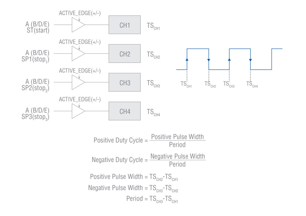
Fig. 58 Duty cycle measurement

This is not a back-to-back measurement, meaning that there is a dead-time of 50 ns or 1 us (depending on particular model and licenses installed) between the samples. 1 signal can be measured in parallel. Up to 16 million samples total can be measured in a single measurement session.

Rise Time, Fall Time, Rise-Fall Time

By convention, rise/fall time measurements are made with the trigger levels set to 10% (start) and 90% (stop) of the maximum pulse amplitude. For ECL circuits, the reference levels are instead nominally 20 % (start) and 80 % (stop). In this case one can use Relative Trigger Levels mode and set trigger levels to 20% and 80% respectively.

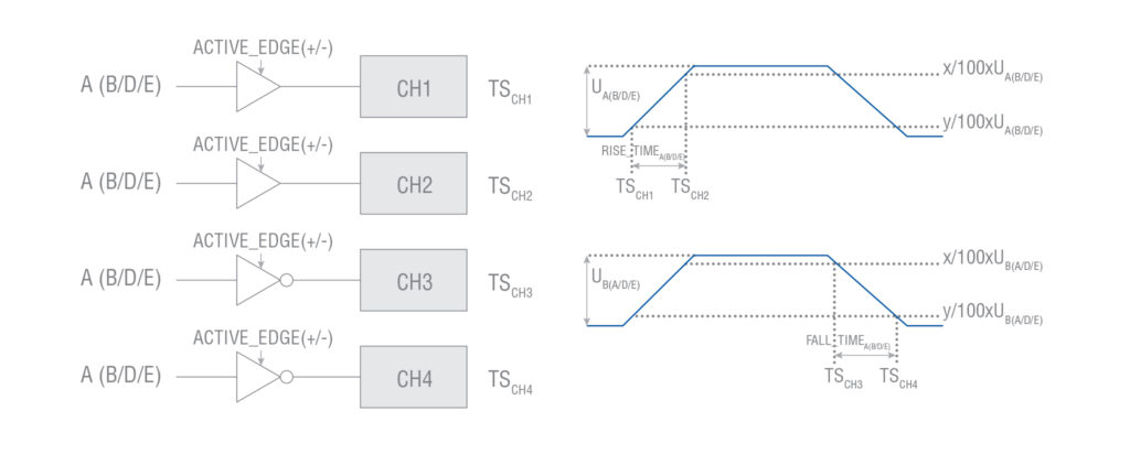
Fig. 59 Rise Time and Fall Time measurement

These are not a back-to-back measurement, meaning that there is a dead-time of 50 ns or 1 us (depending on particular model and licenses installed) between the samples.

Rise Time and Fall Time functions can measure up to 2 input signals in parallel for CNT-104S, CNT-104R, 1 - for CNT-102, with up to 16 million samples per session total.

Rise-Fall Time function (only available for CNT-104S, CNT-104R) can measure only 1 signal but provides both rise and fall time at once. Up to 8 million samples total can be measured in one measurement session.

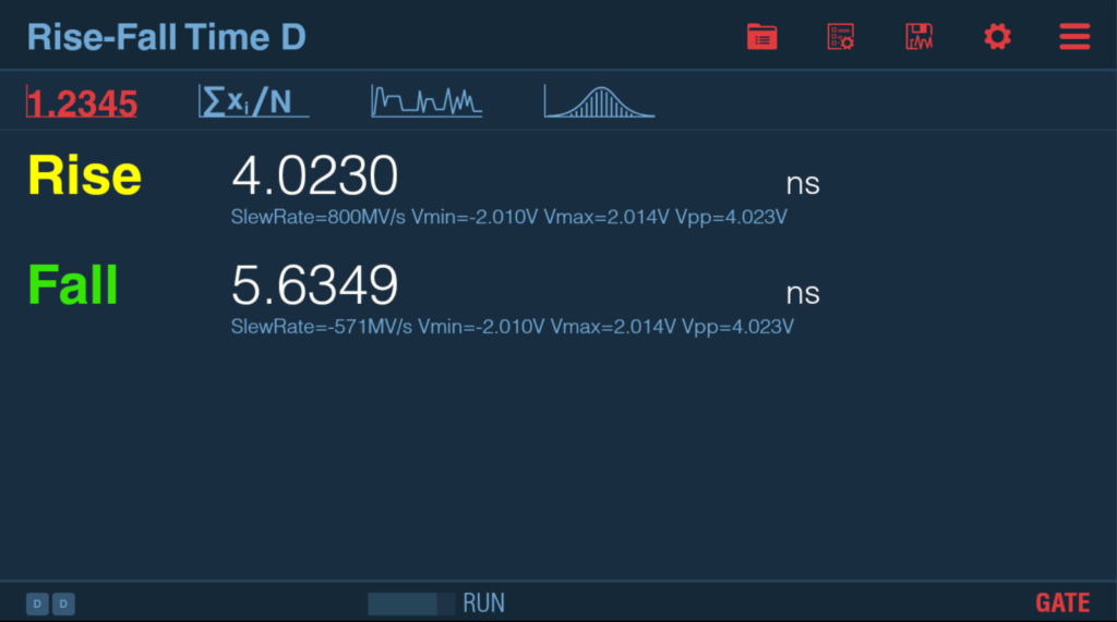
Fig. 60 Rise Time vs Rise-Fall Time

Positive and Negative Slew Rate

Slew rate is the speed of voltage change on pulse positive or negative edge. Hence, Positive and Negative Slew Rate are based on Rise Time and Fall Time measurements, the following formulae are applied (1):

(1)\[ \begin{align}\begin{aligned}PositiveSlewRate = RiseTime / ( 0.8 * ( V_{max}-V_{min} ) )\\NegativeSlewRate = FallTime / ( 0.8 * ( V_{max}-V_{min} ) )\end{aligned}\end{align} \]

Fig. 61 Positive and Negative Slew Rate

Totalize

Totalize functions count the number of trigger events on instrument inputs. There are few modes Totalize can operate in. See next sections for details. In each of these modes the user can choose between Totalize, Totalize X+Y, Totalize X-Y or Totalize X/Y.

Manual Totalize

If neither Start nor Stop Arming is used, Totalize operates in so-called Manual Totalize mode.

In this mode RESTART button start counting trigger events, while HOLD/RUN button is used to pause and resume the counting. Sample Interval setting has no effect, samples are generated each 100 ms.

Timed Totalize

Setting Start Arming Source to Off and Stop Arming Source to Timer enables so-called Totalize Timed Mode.

In this mode RESTART button start counting trigger events for time duration set by Sample Interval (which defines the length of Totalize Gate). Single sample is generated after the end of the Gate.

Armed Totalize

If both Start Arming Source and Stop Arming Source are set, then start and stop arming events define start and stop of Totalize Gate for each Sample (Arm On setting is ignored, the instrument uses arming in Sample implicitly).

See Arming for details on this Totalize mode.

Voltage

The instrument measures the voltage by searching the minimum and maximum signal levels. See Voltage measurement principles for details.

Vmin, Vmax and Vpp functions allow measuring voltage on 4 input signals in parallel for CNT-104S, CNT-104R, 2 - for CNT-102. Vminmax allows only one input but provides both – min and max – at the same time. Resolution is 1 mV, up to 16 million samples can be acquired in one measurement session.

Measurement cheat-sheet

Generic hints

• Whenever you find yourself in trouble while setting up the measurement – use Autoset:

  • Connect the signals,Choose measurement function/inputs,Choose Sample Count and Sample Interval,

  • Press Autoset button,

And it will find proper settings for most cases when measuring continuous signals.

• Use Auto choice for settings items unless you understand the implications of selecting other option.

• Settings → User Option → Recall Defaults will reset measurement settings to Defaults.

• Save complex measurement configurations as Presets (Settings → Measurement Presets or dedicated icon on measurement screen). In this case you can easily recreate the same measurement setup if you need it later.

• Make sure input circuits are setup appropriately:

  • Use Auto-trigger for signals above 100 Hz, otherwise make sure Absolute trigger level is set. appropriately (prefer using Autoset for low frequency signal – it will set trigger levels for you).Make sure input impedance is set correctly.Use only DC coupling for low frequency signals and rely on Autoset to setup proper trigger levels.Keep Preamp OFF, except for extremely low input signal levels (below 50 mVrms).Keep Attenuation 1x, except for signals with amplitudes above exceeding +/- 5V.

  • Keep Filter OFF, except for low frequency sine wave signals (below 100 kHz).

• Settings → Advanced → Voltage Mode should be set to Normal, except for signals below 100 Hz. For signals below 100 Hz please use Autoset to let the counter select best voltage mode for you. Set Voltage mode explicitly only if Autoset fails to find appropriate instrument setup (e.g. for not continuous signals)

Measuring 1 PPS

Hints:

• Set DC on inputs 1 PPS signals are connected to,

• Select measurement function and inputs,

• Set Sample Interval to 0,

• Use Autoset or set Trigger Mode to Manual and set Trigger Level to the middle of 1 PPS signal voltage range.

Same is most of the time true for signals below 100 Hz.

Measuring single cycles or pulses

Hints:

• Set DC on the inputs, which the signals are connected to,

• Select:

  • Period Single for measuring single cycle frequency period, or

  • Time Interval Single for measuring intervals between events, or

  • Totalize for counting events, or

  • Any function from Pulse group for measuring pulse characteristics.

Please note: using other functions will not give reliable results for single cycles/pulses.

• Set Trigger Mode to Manual and set Trigger Level to the middle of signal voltage range.

Please note: auto-trigger won’t work for single cycles/pulses.

Measuring Frequency/Period

See Measuring 1 PPS if signal is below 100 Hz.

Hints:

• The basic setting Sample Interval in the Measurement menu is central to all Frequency related measurement. This setting means the same as Measuring time, or Gate time, used by other counter manufacturers.

A long Sample Interval (Gate time) increases resolution (counting during a longer time) but decreases measurement speed. The Sample Interval is always a compromise between how many digits you want to read, and how fast you want to take your frequency samples. For normal bench use – 200 ms is a good choice, because it is hard for the eye to follow faster changes in the displayed value.

The instrument will give 12-13 digits resolution with 1 s Sample Interval, 9 digits with 1 ms Sample interval, and 6 digits with 1 μs Sample Interval

• Use AC Coupling because possible DC offset is normally undesirable.

• Use Trigger Mode Auto and/or Autoset.

• Use Preamp ON for signals with amplitudes below 200 mVpp.

Please note: amplifying the signal also amplifies the noise.

• Sample Interval of 200 ms is a reasonable tradeoff between measurement speed and resolution on the bench.

Time measurements of continuous signals

Hints:

• Use DC coupling.

• High signal level, and Steep signal edges.

Jitter measurements

Statistics provides an easy method of determining the short term timing instability, (jitter) of pulse parameters.

Note: that the measured pulse parameter should be a single cycle value, whether it is period, or pulse width.

Single cycle jitter

Single cycle jitter made on random samples of single periods, is usually specified with its rms value, which is equal to the standard deviation based on single measurements. The instrument can then directly measure and display the rms jitter. Jitter can also be expressed as peak-to-peak value, which is also displayed in the Statistics screen.

Cycle-to-cycle jitter

Cycle- to-cycle jitter demands zero dead-time measurements without gaps and can be made on input signals with a jitter frequency of up to 20 MHz for CNT-104S, CNT-104R and FTR-210R with Options 230, 122F. There is currently no dedicated measurement function, but the raw data of a Period Average measurement, with Sample Interval of 0 or down to 50 ns or 1 us (depending on particular model and licenses installed), could be exported to e.g. Matlab or Excel for “number crunching” and analysis.

Wander measurements

Wander measurements, which is a “slow jitter” measurement with jitter frequencies <10 Hz is made by using the TIE function, which compares the accumulated period phase drift, with the ideal phase from an ideal clock.

Deterministic jitter

Deterministic jitter is revealed in the Distribution graph, which will show underlying noise sources in a clear way. For example a sine modulated noise source would give a bathtub shape, a pulse modulated noise source would give a twin peak shape, and a measurement of a source containing not one, but two, fundamental frequencies will be displayed as “double hump”.

Frequency Modulated Signals

A frequency modulated signal is a carrier wave signal (CW frequency = f0) that changes in frequency to values higher and lower than the frequency f0. It is the modulation signal that changes the frequency of the carrier wave.

The instrument can accurately measure:

• f0 = Carrier frequency.

• fdev = Frequency deviation = (fmax -fmin)/2. And via the timeline graph, you will also get a good indication of the modulation frequency fmod

Initial capture settings

The optimum settings is to find a balance between large enough sample intervals to achieve high resolution per individual frequency sample, max. 10% of the Frequency deviation.

And small enough Sample intervals to capture enough frequency samples per modulation cycle for good graph visibility.

A rule of thumb is that the number of samples per modulation cycle should be >10, for good graphical view of the modulation signal, and acceptable error of fmax and fmin

Example: 10 kHz modulation frequency (100 us modulation cycle) of a 200 MHz carrier with 200 kHz deviation (0.1% modulation).

Set Sample interval to 10 μs (10% of the modulation cycle). Set Sample Count (N) to 100 (to cover 10 modulation cycles).

Now every frequency sample will have a resolution of (10 ps/10 μs) x 200 MHz = 200 Hz.

This resolution is 1000 times better than the frequency deviation.

Start measurement and view the Timeline graph, which will show10 modulation cycles, with 10 samples per modulation cycle.

To improve the graphical experience, lower Sample Interval to 1 μs (1% of the modulation cycle), and increase Sample Count to 1000.

Now each frequency sample has a resolution of (10ps/1μs) x 200 MHz = 2 kHz. Still with a lot of margin to deviation.

You may want to play around with the Sample Interval and Sample Count setting until you have found your optimum view of the FM signal (no of displayed mod. cycles).

Carrier Wave Frequency f0

To determine the carrier wave frequency, just look at fmean which is best approximation of f0.

Ideally the sum of all Sample Intervals should be selected to cover an integer number of modulation periods. This way the positive frequency deviations will compensate the negative deviations during the measurement.

Example: If the modulation frequency is 1 kHz, the Sample Interval 10 μs and N = 1000 will make the instrument measure exactly 10 complete modulation cycles. A bad combination of Sample Interval and N would worst case mean that exactly half a modulation cycle is uncompensated for, giving a max. error for a sine modulation of:

f0 – fmean = Δfmax / (sample int.) x N x fmod x π

For very accurate measurements of the carrier wave frequency f0, make an extra measurement session and set Sample Interval as close as possible to an integer number of modulation cycles, and increase the number of samples substantially. A worst case error of half a modulation cycle means far less in a million cycles compared to 10 cycles.

Frequency deviation fmax - f0

Read the max, min, and mean frequency values from statistics screen or beneath the graph and calculate fdev as either:

• fmax – fmean

• fmean – fmin

• fp-p/2

These three values should be exactly the same for an ideal sine wave or square wave modulation.

Modulation frequency fmod

The modulation frequency is easiest found by visual estimate in the graph on screen by using Cursors. Place one cursor on the beginning of the first modulation cycle and the other – on the end of the last modulation cycle. If the end point time difference between cursors is T seconds and the exact integer number of modulation cycles between cursors is M, the modulation frequency is:

fmod = M/T

Errors in fmax, fmin, and fp-p

A too large Sample Interval compared to the modulation cycle time leads to an averaging error that will underestimate the true deviation. A Sample interval corresponding to 10% of the modulation cycle, or 36° of the modulation signal, leads to an error of approx. 1.5%.

If that error is not acceptable, decrease the Sample Interval to make more samples than 10 during the modulation cycle.

Frequency profiling

Profiling means measuring and plotting frequency variation versus time. Examples are measuring warm-up drift in signal sources over hours, measuring the linearity of a frequency sweep during seconds, VCO switching characteristics during milliseconds, or the frequency changes inside a “chirp radar” pulse during sub-microseconds.

The instrument can handle many profiling measurement situations with some limitations. In profiling applications, the instrument acts as a fast, high-resolution sampling front end, storing results in its internal memory. These results are later displayed on screen and/or transferred to the controller for analysis and graphical presentation.

You must distinguish between two different types of measurements called free-running and repetitive sampling.

Free-Running Measurements

Free- running measurements are performed over periods down to the sub-microseconds range, e.g., to measure initial drift of a signal generator or oscillator, to plot linearity of a sweep signal ramp, or to measure short-term stability down to microsecond averaging times. In these cases, measurements are performed at user-selected Sample Intervals, and performed as gap-free measurements in the range 50 ns or 1 us (depending on particular model and licenses installed) to 1000 s.

Just start the block measurement and view the profile in the graph presentation mode.

Repetitive Sampling Profiling

The measurement setup just described will not work when the profiling demands less than 50 ns or 1 us (depending on particular model and licenses installed) intervals between samples.

How to do a VCO step response profiling with 50 samples during a time of 1 us.

This measurement scenario means that you need to come to 20 ns between samples (50 points * 20 ns = 1 ms observation time).

You will need a repetitive input step signal, and you have to repeat your measurement 50 times, taking one new sample per cycle. And every new sample should be delayed 20 ns with respect to the previous one.

Profiling can theoretically be done manually, but the best would be to perform this series of measurements with a dedicated program on PC, controlling the instrument and collecting data from it remotely.

The following are required to setup a measurement:

A repetitive input signal (e.g., frequency output of VCO). An external SYNC signal (e.g., step voltage input to VCO). Use of start arming delay (20, 40, 60 ns, etc). See Fig. 62 for a test setup diagram.

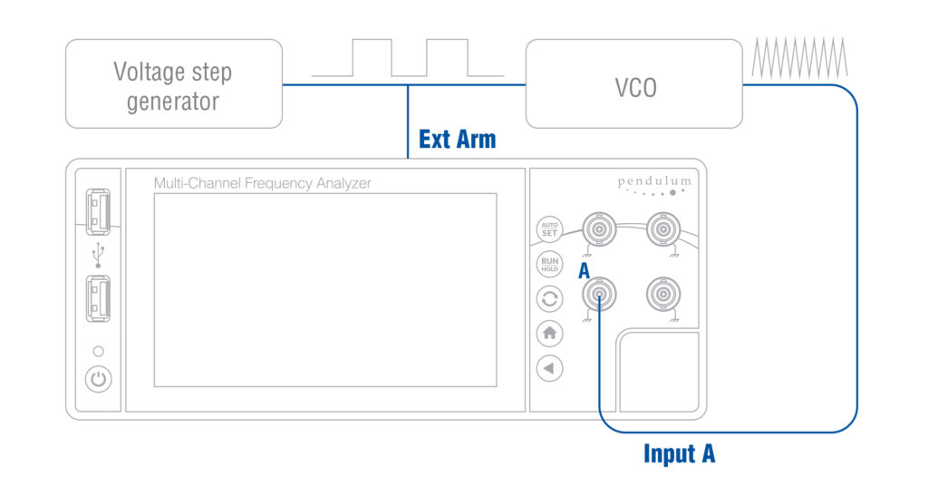
Fig. 62 Setup for transient profiling of a VCO.

Vrms

When the waveform (e.g. sinusoidal, triangular, square) of the input signal is known, its crest factor, defined as the quotient (Q_CF) of the peak (V_p) and RMS (V_rms) values, can be used to set the constant K in the mathematical function K*X+L. The display will then show the actual Vrms value of the input signal, assuming that V_pp is the main parameter.

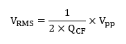
Example: A sine wave has a crest factor of 1.414 (\(\sqrt{2}\)), so the constant in the formula above will be 0.354.

Other features

Hold-off

Hold- off function allows to insert dead-time into input trigger circuit which effectively acts as a digital lowpass filter. Hold-off can be set to 0 (Hold-off OFF) or in the range [20 ns .. 2.683 s] which correspond to low-pass filter frequency from 100 MHz down to 0.5 Hz.

Setting Hold-off to approx. 75% of the cycle time of the signal allows to inhibit erroneous triggering for noisy signals.

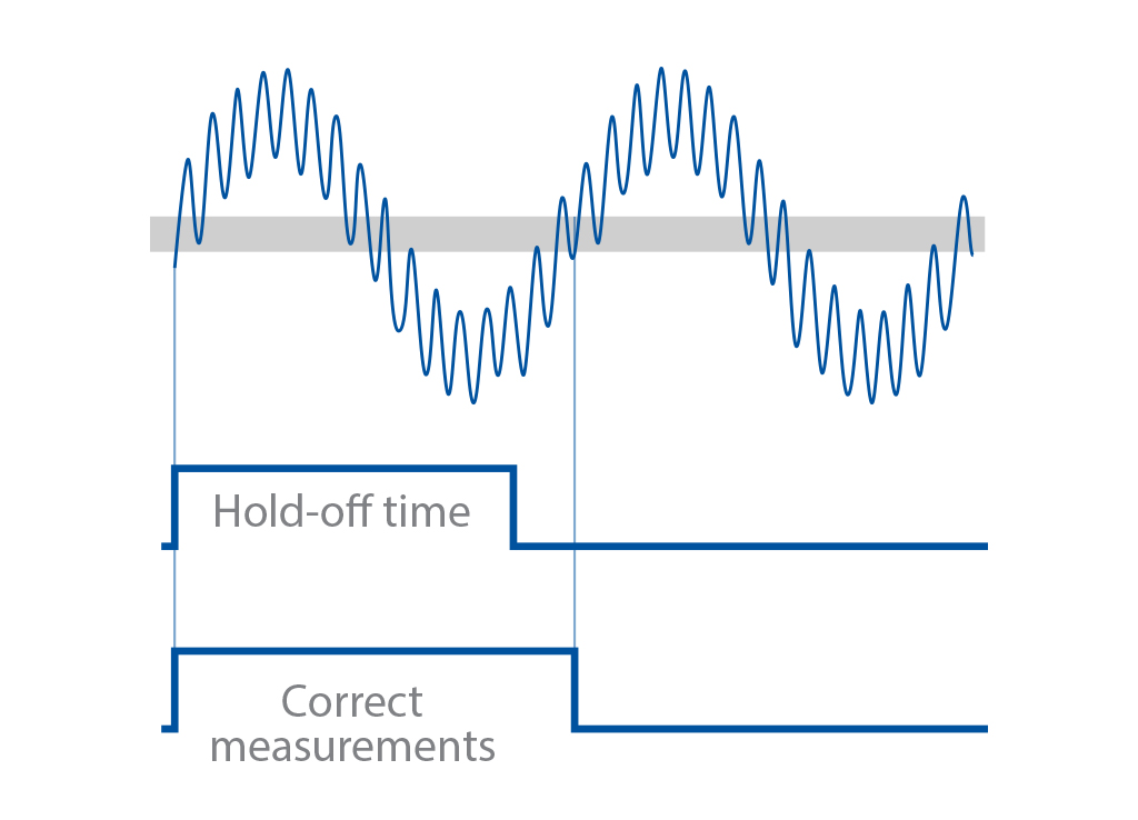
Fig. 63 Using hold-off as a Digital LP filter to cope with erroneous triggering on noisy signal

Hold-off is also an effective measure to cope with contact bouncing on the front of the signal under test.

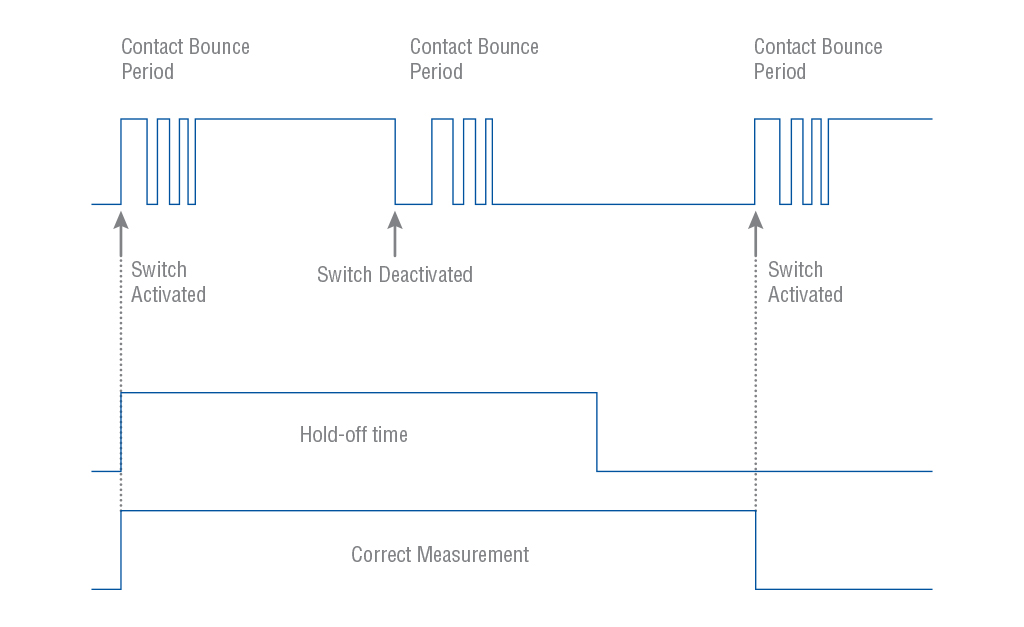
Fig. 64 Using Hold-off to cope with switch bounce effect

You should be aware of a few limitations to be able to use the Hold-off feature effectively and nambiguously. First you must have a rough idea of the frequency to be measured. A cutoff frequency that is too low might give a perfectly stable reading that is too low. In such a case, triggering occurs only on every 2nd, 3rd or 4th cycle. A cutoff frequency that is too high (>2 times the input frequency) also leads to a stable reading. Here one noise pulse is counted for each half-cycle.

Timeout

The instrument ends measurement when all requested samples have been collected. However, if signal is absent (or lost) on one of the inputs used for the measurement – timestamps from this channel will never come and instrument will wait forever unless measurement is stopped explicitly.

However, in many cases this is undesirable behavior. For example in an automated test system when absence of signal can be a result of a wrong test setup or device under test malfunction, it is would be a waste of time to wait until the expected end of a long measurement to discover that one of the signals is just missing.

This is where Timeout function comes to help. If Timeout is ON, the measurement will end in case there are no samples from one of measurement inputs for the time duration set by Timeout Time.

Calibration

Internal Calibration

The instrument has a possibility to compensate for some internal sources of error by the means of internal calibration. This procedure doesn’t require any external signal, the instrument can perform it automatically.

Performing internal calibration before the start of measurement helps getting maximum accuracy and best resolution. However, because internal calibration takes up to 2 s it has impact on measurement speed which might be important in automated test systems. Hence, the instrument allows to choose the schedule of internal calibration. Summarizes available options.

Mode	Description
Every 30 minutes	The instrument performs internal calibration every 30 minutes between successive measurements or when it is idle. This is the default option which provides the best trade-off between accuracy, resolution and average measurement speed.
Before every measurement	The instrument performs internal calibration before each timing measurement to ensure best resolution and accuracy. This results in additional time overhead of around 2 s per measurement session. If such overhead is not critical – this is the recommended choice.
Once (after warm-up)	The instrument performs internal calibration only once – after the instrument has warmed up. This guarantees no calibration overhead, but resolution will deteriorate over time.

Table 4. Internal Calibration Modes

To provide maximum flexibility, the instrument also provides the possibility to perform internal calibration explicitly. This is especially useful when Interpolator Calibration Mode is set to Once.

All above can be configured under Settings → Advanced section (see Fig. 65).

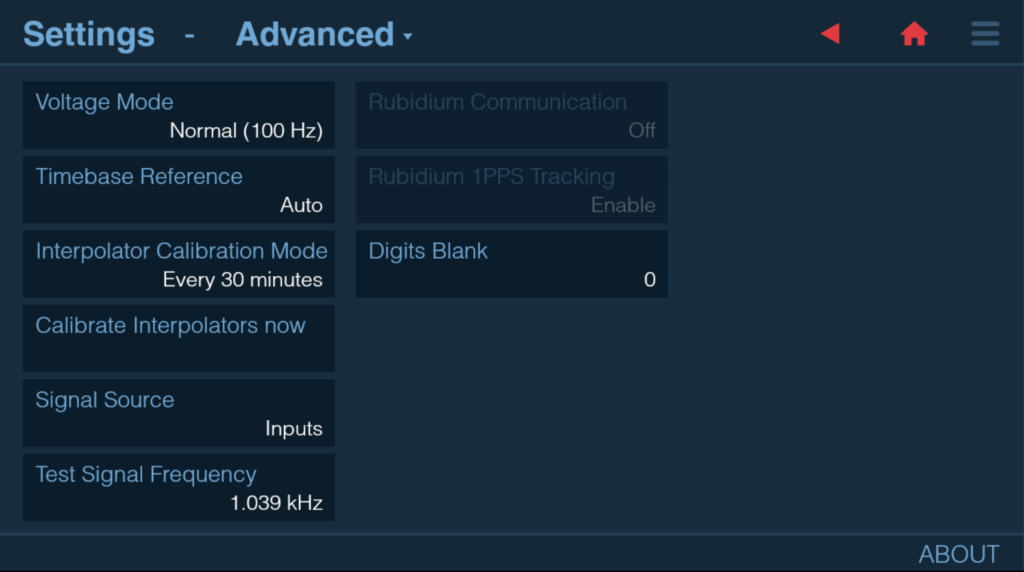
Fig. 65 Internal Calibration configuration

Timebase Calibration

Note

For FTR-210R GNSS disciplined Frequency and Time References and CNT-104R with GNSS option, timebase calibration is not required unless they are constantly used in Hold-over or Manual Hold-over modes

For increasing measurement accuracy, a good reference source can be used for timebase calibration. Connect the source to Input A, select Settings→Timebase Calibration, choose reference frequency and start the procedure. It is possible to interrupt the process midway, re-apply result from previous calibration or reset to factory calibration setting.

Note

Pictures below illustrate display of CNT-104S model.

For CNT-102, channels D, E are not available and areas, fields and graphical objects for corresponding to these channel are not present. Up to 2 signals can be measured in parallel.

For FTR-210R, channels B, D, E, C are not available and areas, fields and graphical objects for corresponding to these channel are not present. Only one signal can be measured in parallel.

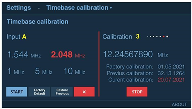
Fig. 66 Timebase Calibration menu

Voltage Calibration

For increasing accuracy of voltage measurements and manual trigger level setting accuracy, a good source of DC voltage can be used for voltage calibration. Open Settings → Voltage menu, select the input to be calibrated and follow the instructions.

Note

Pictures below illustrate display of CNT-104S model.

For CNT-102, channels D, E are not available and areas, fields and graphical objects for corresponding to these channel are not present. Up to 2 signals can be measured in parallel.

For FTR-210R, channels B, D, E, C are not available and areas, fields and graphical objects for corresponding to these channel are not present. Only one signal can be measured in parallel.

Fig. 67 Voltage Calibration menu

Note

Voltage calibration sets inputs to 1 MOhm impedance.

Mathematics

The instrument can use five mathematical expressions to process the measurement result before it is displayed:

• K×X+L

• K/X+L

• (K×X+L)/M

• (K/X+L)/M

• X/M-1

Select Settings -> Mathematics to enter the mathematics submenu.

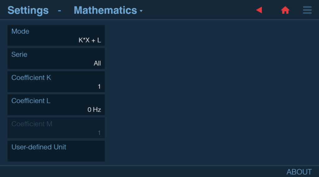
Fig. 68 Mathematics menu

The default values of K (Scale factor), L (Offset) and M (Reference value) are chosen to 1, 0 and 1 respectively, so that the measurement result is not affected directly after activating Math. Recalling the default setting will restore these values as well.

It is possible to apply Mathematics function to all measurement series or to selected one.

When Mathematics is turned on, the instrument status bart shows MATH indicator.

Example use cases

If you want to observe the deviation from a nominal frequency, for example 10 MHz, instead of the absolute frequency itself, you can do like this:

• Select Math

• Select the expression K×X+L

• Select K = 1 (if not already set)

• Select L = -10 MHz

• Now the display will show the deviation from the value you have just entered.

By changing the constant K you can scale the result instead. Set for example K = 60 to convert Frequency in Hz to RPM (revolutions per minute) from rotation transducers.

Use the expression X/M-1 if you want the result to be displayed as a relative deviation. The result will be displayed as

%, ppm, ppb, or as a dimensionless number like +1.2345E-12

Limits

Limits feature is used for setting numerical limits and selecting the way the instrument will report the measurement results in relation to them.

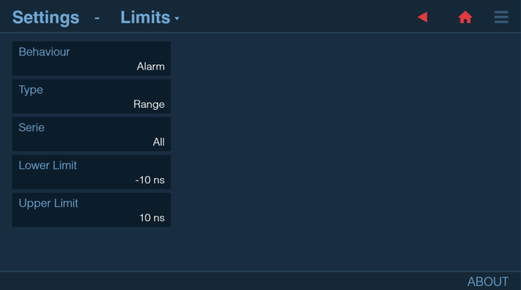
Fig. 69 Limits configuration

Limit Behavior setting defines how the device will react on limits:

• Off – limits are not checked.

• Capture – only samples meeting the limit criterion are captured, the rest are discarded. Limit status is displayed.

• Alarm – all samples are captured; limit status is displayed.

• Alarm Stop – measurement session stops if measured value doesn’t meet the limit criterion.

Limit Type:

• Above – results above set Lower Limit will pass.

• Below – results below set Upper Limit will pass.

• Range – results within the set limits will pass.

Limits can be applied to all measurement series or to selected one, depending on user’s choice.

When Limit Behavior is not Off, the instrument status bar shows LIM. It will change to LIM! if at least one sample didn’t meet set Limit criterion during measurement session.

Numeric, Graph and Distribution screens will also have additional Limit indicators displayed.

Note

Pictures below illustrate display of CNT-104S model.

For CNT-102, channels D, E are not available and areas, fields and graphical objects for corresponding to these channel are not present. Up to 2 signals can be measured in parallel.

For FTR-210R, channels B, D, E, C are not available and areas, fields and graphical objects for corresponding to these channel are not present. Only one signal can be measured in parallel.

Fig. 70 Limits display

Pulse Output (option)

Note

License is needed to unlock Pulse Output functionality in the instrument.

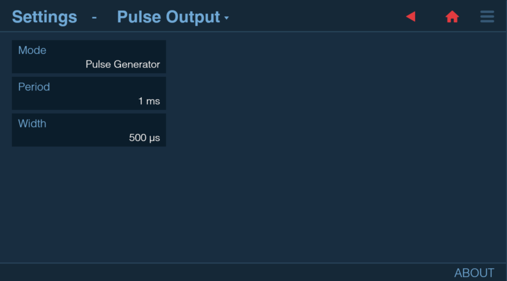
Fig. 71 Pulse Output configuration

Pulse Output is located on rear panel of the instrument and can be used for one of the following purposes:

• Pulse Generator. Pulse period can be selected from the range [10 ns .. 2.147 s] in 2 ns steps, pulse width – in the range [6 ns .. 2.147 s] in 2 ns steps.

• Gate Open. Indicates if measurement is in progress.

• Alarm Out. Indicates when Limits Alarm is active. Can be selected between Active High and Active Low

Irrespective to the selected mode, the amplitude of Pulse Output signal is set to TTL levels into 50 Ohm termination

Network

The instrument supports wired 10/100/1000 Mbps connection as well as wireless (via external USB Wi-Fi adapter).

It has IPv4 support and can be configured in either Static or Dynamic (DHCP) mode. If Static mode is selected, user is expected to manually enter IP address, Network mask and Gateway. For Dynamic mode, these fields are read-only and display IP address, network mask and gateway that are currently in use.

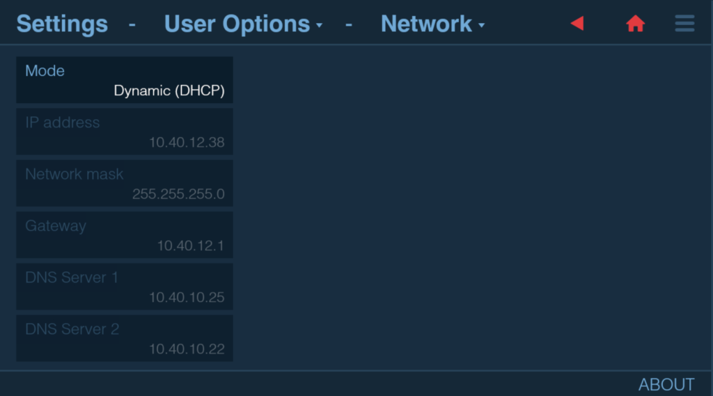
Fig. 72 Network configuration

Web Interface

The instrument has built in web server that provides Web Interface allowing to see the instrument screen and control it remotely, download files and upgrade firmware.

Note

Pictures below illustrate display of CNT-104S model.

For CNT-102, channels D, E are not available and areas, fields and graphical objects for corresponding to these channel are not present. Up to 2 signals can be measured in parallel.

For FTR-210R, channels B, D, E, C are not available and areas, fields and graphical objects for corresponding to these channel are not present. Only one signal can be measured in parallel.

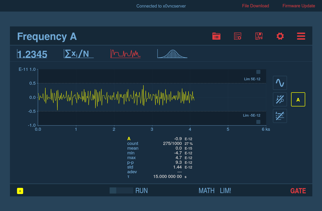
Fig. 73 Web Interface

Fig. 74 Firmware Update page of the Web Interface

Fig. 75 File Download page of the Web Interface

VNC

The instrument also exposes VNC server on port 5901 which allows remote access and control. One can use any VNC client software on PC, mobile phone or tablet.

Front USB ports

Front panel USB ports can be used for connecting:

• Peripherals (PC keyboard and mouse) which complement the touch screen interface.

• USB storage for saving measurement results, presets or upgrading firmware.

• Wi-Fi adapter for enabling wireless networking.

File Manager

The instrument has built-in File Manager accessible via Settings → User Options → File Manager or dedicated icon on measurement screen.

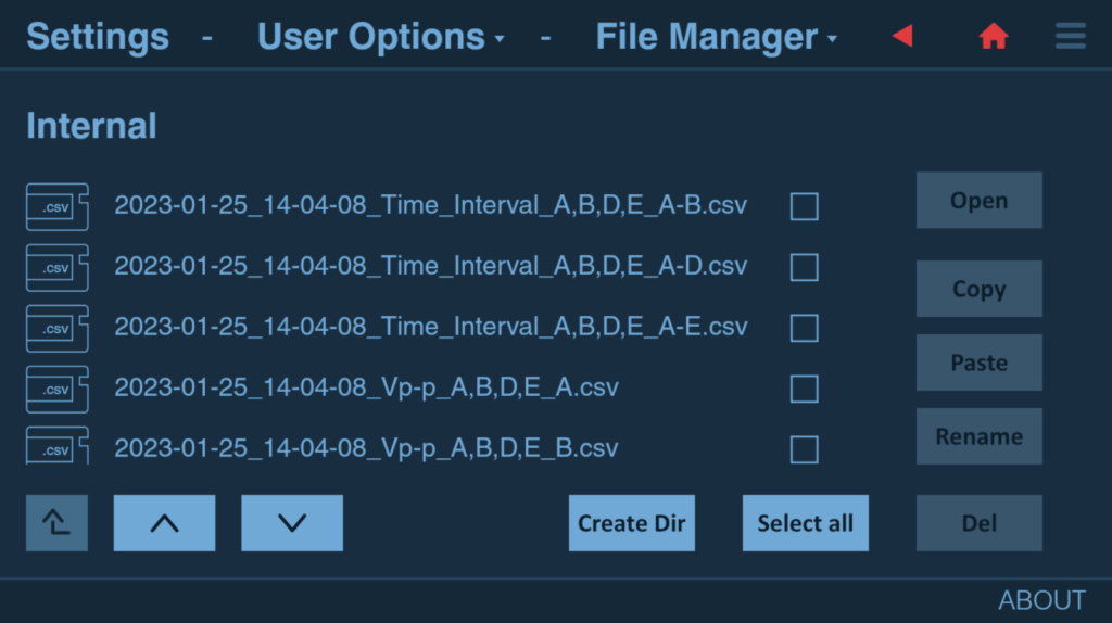
Firmware Update

There are 2 ways of updating firmware of the instrument:

Update via Web Interface (preferred):

• Download SW update file (it has .swu extension) to your PC

• Connect the instrument to LAN: either via ethernet cable or use supported Wi-Fi dongle to connect via Wi-Fi

• On the instrument open Settings -> User Options -> Network to check or set current IP address

• On PC, open web browser and put the instrument address to adress field. The instrument’s Web Interface will open

• Click Software Update link on top right and follow the instructions

Update via USB stick:

• Copy SW update file (it has .swu extension) to USB stick

• Insert USB stick to one of the instrument front panel USB ports

• On instrument’s Open Settings -> User Options -> Firmware Update to open Firmware Update screen

• On instrument’s Firmware Update screen tap/click on SW update file. SW update will start. No progress indication will be displayed – wait until the instrument reboots

Installing license

• Put License File on USB stick

• Plug it to one of front USB ports

• Navigate to Settings → User Options → Import License

• Select License to be imported

Performance Check

General Information

WARNING: Before turning on the instrument, ensure that it has been installed in accordance with the Installation Instructions outlined in Chapter 1 of the User’s Manual.

This performance procedure is intended for:

• checking the instrument’s specification.

• incoming inspection to determine the acceptability of newly purchased instruments and recently recalibrated instruments.

• checking the necessity of recalibration after the specified recalibration intervals.

NOTE: The procedure does not check every facet of the instrument’s calibration; rather, it is concerned primarily with those parts of the instrument which are essential for determining the function of the instrument.

It is not necessary to remove the instrument cover to perform this procedure.

Preparations

Power up your instrument at least 30 minutes before checking to let it reach normal operating temperature. Failure to do so may result in certain test steps not meeting equipment specifications.

Test Equipment

Type of Equipment	Required Specifications
Reference Oscillator	10 MHz, 1×10-8 (e.g. 6688) for calibrating the standard TCXO oscillator 10 MHz, 1×10-9 (e.g. 6689) for calibrating Opt 30 & Opt 40 (OCXO)
Voltage Calibrator	DC -50 V to +50 V (e.g. Fluke 5500) for calibrating the built-in voltage reference, alternatively corresponding DC power supply + DVM with uncertainty <0.1 %
LF Synthesizer	Square/ Sine up to 10 MHz, 10 VRMS
Pulse Generator	2 ns rise time, 5 V peak, >10 MHz, continuous & one-shot trigger
Oscilloscope	1 GHz, <3% voltage uncertainty
RF Signal Generator	0.1 to 3, 10, 15, 20, or 24 GHz dep. on RF input, <1dBm level uncertainty, 10 MHz ext.ref.
Power Splitter	50 Ohm 6dB BNC
T-piece	BNC
Termination	50 Ohm feed through BNC
Low-pass Filter	50 kHz (for 1 MOhm) load
BNC Cables	Approx. 10 pcs of suitable lengths

Table 5. Recommended equipment for calibration and performance check.

Internal Self-Tests

Internal self-tests are run on every instrument power up. In case of a failure information message box appears described the type of the error.

Front Panel Controls

Touch Panel and Keyboard Test

• Press Settings icon on top right. Open User Options → Recall Defaults. Confirmation dialog will appear.

• Press Yes.

• Press BACK hard button. Main Settings screen will appear.

• Press Advanced, then press Signal Source and select Test.

• Press ABOUT in bottom right corner. About box will appear.

• Press OK.

• Press HOME hard button. Measurement screen will appear. Frequency around 1 MHz will be measured.

• Press HOLD hard button. Measurement will be put in HOLD after current one finishes.

• Press RESTART hard button. Instrument will perform single measurement.

• Press Measurement Function name in top left corner. Function selection dialog will appear.

• Select Period → Period Single → A, B.

• Press OK. Measurement screen will appear.

• Press AUTOSET hard button. Autoset progress dialog will appear followed by “Autoset finished” notification.

Short Form Specification Test

Sensitivity and Frequency Range for measurement inputs

• Recall Defaults

• Select Frequency A.

• Select 50 Ω input impedance, 1x attenuation, Manual Trigger Levels and Absolute Trigger Level A 0V.

• Select Preamp ON

• Connect a signal from a HF generator to a BNC power splitter.

• Connect the power splitter to Input A of your counter and an oscilloscope. Set the input impedance to 50 Ω on the oscilloscope.

• Adjust the amplitude according to the following table. Read the level on the oscilloscope. The timer/counter should display the correct frequency.

• Repeat the measurements and input settings above for inputs B, D, E (on CNT-104S, CNT-104R) or B (on CNT-102)

Table 4 Sensitivity of measurement inputs at various frequencies

Frequency (MHz)	Level (mVrms)	Level (dBm)	Pass/Fail
10	15	-23
50	15	-23
100	15	-22
200	15	-23
300	25	-19
400	35	-16

Sensitivity and Frequency Range for RF Input (Input C)

To verify the specifications of the different RF prescalers, use the following basic test setup:

• Connect the output of a signal generator covering the specified frequency range to the RF input (C) of the instrument.

• Connect the 10 MHz REF OUT from the generator to the EXT REFon the rear panel of the instrument. Choose External in Settings → Advanced → Timebase Reference.

• Select Frequency C as Measurement Function.

• Generate a sine wave in accordance with the data in the relevant table (Table 7, Table 8).

• Verify that the instrument is counting correctly. (The last digits will be unstable).

Table 5 RF input sensitivity, Option 10 (3 GHz)

Frequency GHz	Amplitude dBm
0.1-0.3	-21
0.3-2.5	-27
2.5-2.7	-21
2.7-3.0	-15

Table 6 RF input sensitivity, Option 110 (10, 15, 20 or 24 GHz)

Frequency GHz	Amplitude dBm
0.15-0.3	-15
0.3-0.5	-21
0.5-7.5	-27
7.5-20	-24
20-22	-21
22-24	-15

Voltage

• Recall Defaults.

• Select Vpp A

• Select DC coupling and Filter 10 kHz. Do not apply an input signal to Input A yet.

• The display should now indicate (disregard the main parameter Vpp): Vmin= 0 ± 0.015 V and Vmax= 0 ± 0.015 V

• Adjust the current limit of the DC voltage source to <200 mA.

• Connect +2.500 Vdc to Input A, using the external 50 kHz low-pass filter on the input.

• The display should now indicate: Vmin = 2.500 ± 0.040 V and Vmax = 2.500 ± 0.040 V Repeat the measurement with inverted polarity.

• Select Input A and select 10x.

CAUTION: Before the next step, make sure the input impedance is still 1 MΩ. Applying more than 12 V without proper current limiting may cause extensive damage to the main PCB, if the impedance is set to 50 Ω.

• Change the DC level to +50.00 V.

• The display should now indicate: Vmin = 50.00 ± 0.65 V and Vmax = 50.00 ± 0.65 V Repeat the measurement with inverted polarity.

• Disconnect the DC voltage from Input A. Remove the external low-pass filter.

• Select Input A and select 1x.

• Connect the LF generator to Input A, and set an amplitude of 4.000 Vpp and a frequency of 100 kHz. Verify the Amplitude with a good Voltmeter

• The display should now indicate: 4.000 ± 0.150 Vpp.

• Select Input A and select 10x.

• Change the amplitude to 18.00 Vpp.

• The display should now indicate: 18.00 ± 1 Vpp. Disconnect the LF generator from Input A.

• Select Input A and select 1x, 50 ohm, and Filter = OFF.

• Connect the RF generator to Input A and set an amplitude of 4.000 Vpp and a frequency of 100 MHz. Verify the amplitude on an oscilloscope.

• The display should now indicate: 4.000 ± 0.40 Vpp. Select Input A and select 10x.

• Change the amplitude to 18.00 Vpp.

• The display should now indicate: 18.00 ± 2.2 Vpp

• Proceed by repeating the measurements for inputs B, D, E (on CNT-104S, CNT-104R) or B (on CNT-102), as described above for Input A.

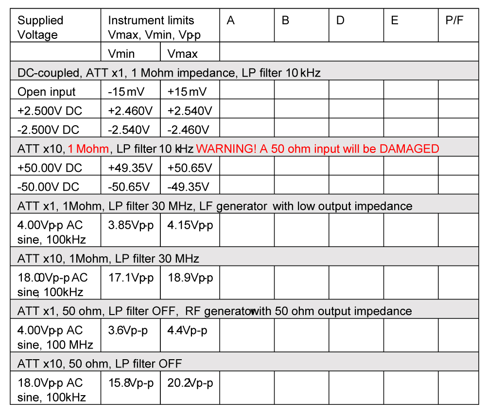
Reference Oscillators

X- tal oscillators are affected by a number of external conditions like ambient temperature and supply voltage. Aging is also an important factor. Therefore, it is hard to give limits for the allowed frequency deviation. The user himself must decide the limits depending on his application and recalibrate the oscillator accordingly.

To check the accuracy of the oscillator you must have a calibrated reference signal that is at least five times more stable than the oscillator that you are testing. See Table 7-6 and the list of test equipment on page 7-2. If you use a non-10 MHz reference, you can use the mathematics in the timer/counter to multiply the reading.

• Recall Defaults

• Connect the reference to input A

• Check the readout against the accuracy requirements of your application.

Acceptance Test

Table 7 can serve as an acceptance test and gives a worst case figure after 30 minutes warm-up time. All deviations that can occur in a year are added together.

Table 7 Acceptance test for oscillators

Oscillator	Frequency Readout	Suitable Reference	P/F
Standard (TCXO)	10.00000000 MHz + 150 Hz	6688
Option 30 (OCXO)	10.00000000 MHz + 1Hz	6689
Option 40 (OCXO)	10.00000000 MHz + 0.25 Hz	6689

Resolution Test

Note

This test can’t be done on FTR-210R

• Connect the pulse generator to a power splitter.

• Connect one side of the power splitter to Input A on the instrument using a coaxial cable.

• Connect the other side of the power splitter to Input B on the instrument.

Settings for the pulse generator:

• Amplitude = 4 V_pp, (high level +4 V and low level 0 V) Period = approx. 1 ms

• Duration = approx. 50 ns

• Rise time = 2 ns

Settings for the instrument:

• Recall Defaults,

• Select Time Interval Single A, B,

• Set for Inputs A & B: 50 Ω, DC coupling, Manual Trigger Levels,

• Set Absolute Trigger Level A to +1 V,

• Set Absolute Trigger Level B to +1 V,

The standard deviation (std) should be less than 140 ps, corresponding to a resolution of 7 ps per timestamp.

Rear Inputs/Outputs

10 MHz OUT

• Connect an oscilloscope to the 10MHz output on the rear of the instrument. Use a coaxial cable and 50Ω termination.

• The output voltage should be sinusoidal and >1V_p-p, typically 1V_rms.

EXT REF FREQ IN

Note

Not available for FTR-210R GNSS disciplined Frequency & Time Reference

• Recall Defaults.

• Connect a stable 10 MHz signal (e.g REF OUT from another counter/analyzer) to input A. Connect a 10 MHz, 100 mV_RMS, (0.28 Vp-p) signal from the LF synthesizer to EXT REF. Select Ext Ref. from the Timebase Oscillator setting menu

• The display should show 10 MHz.

• Change the external reference frequency to 5 and 1 MHz.

• The counting should continue, and the display should still show 10 MHz.

EXT ARM IN

Note

Not available for FTR-210R GNSS disciplined Frequency & Time Reference

• Proceed from the test above.

• Settings for the pulse generator:

  • single shot pulse,

  • manual trigger,

  • amplitude TTL = 0 – 2 VPP, and

  • duration = 10 ns.

• Connect the pulse generator to Ext Arm Input.

• Set Start Arming to EA on the instrument. The instrument does not measure.

• Apply one single pulse to Ext Arm Input.

• The instrument measures once and shows 10 MHz on the display.

PULSE OUT

• Connect an oscilloscope to the pulse output on the rear panel with a 50 Ω coaxial cable terminated at the scope input with 50 Ω (internally or externally).

• Enter Settings → Pulse Output.

• Set Mode to Pulse Generator. Select Pulse Period and set the value to 1000 ns. Select Pulse Width and set the value to 500 ns.

• The output signal should be a pure square wave signal with 1 MHz frequency and 50 % duty cycle. The rise/fall time should be approximately 2.5 ns. The low and the high level should be <0.2 V resp. >2.4 V.

Measuring Functions

Note

Particular measurement function availability depends on particular model and licenses combination.

• Recall Defaults

• Set Settings → Advanced → Signal Source to Test

• Set Sample Interval to 200 ms

• Set DC, 50 Ω, Manual Trigger Levels, Absolute Trigger Level to 0.5 V for inputs A, B, D, E (on CNT-104S, CNT-104R) or A, B (on CNT-102)

• Go through Measurement Functions from the Table 8 and verify the results.

Note that the results in the table are rounded off and very approximate. Test signal is not synchronized to instrument timebase and can generate Frequencies far from nominal. No tolerances are given for this test.

Measurement Function	Display	Pass/Fail
Frequency A,B, {D,E}	1 MHz
Smart Frequency A,B,{D,E}	1 MHz
Frequency Ratio A,B,{D,E}	1
Period Average A,B,{D,E}	1 us
Smart Period Avg A,B,{D,E}	1 us
Period Single A,B ({D,E})	1 us
Time Interval A,B,{D,E}	>-100 ps, <100ps
Time Interval Single A,B,{D,E}	>-100 ps, <100ps
Acc. Time Interval A,B,{D,E}	>-100 ps, <100ps
Phase A,B ({D,E})	0° (360°)
Acc. Phase A,B ({D,E})	0° (360°)
TIE	0 s
Pos. Duty Cycle A (B,{D,E})	0.5
Neg. Duty Cycle A (B,{D,E})	0.5
Pos. Pulse Width A,B ({D,E})	500 ns
Neg. Pulse Width A,B ({D,E})	500 ns
Rise Time A, B ({D,E})	< 5 ns
Fall Time A, B ({D,E})	< 5 ns
Rise-Fall Time A (B,{D,E})	< 5 ns
Pos. Slew Rate A, B ({D,E})	>350 MV/s
Neg. Slew Rate A, B ({D,E})	<-350 MV/s
Totalize A,B,{D,E}	increments
Totalize X+Y A,B,D,E	increments
Totalize X-Y A,B,{D,E}	0
Totalize X/Y A,B,{D,E}	1
Vmin A,B,{D,E}	0 V
Vmax A,B,{D,E}	2 V
Vp-p A,B,{D,E}	2 V
Vminmax A (B,{D,E})	Vmin=0 V, Vmax=2 V

Table 10. Measurement Functions check

Optional RF Input C

• With an optional RF input (Input C) you will require an external RF source to verify Input C. A simple functional check can be performed by connecting a 1 GHz, -10 dBm signal after selecting Freq C. No other settings need to be changed.

• Read 1 GHz on the display

Check of HOLD OFF Function

• Recall Defaults

• Select Period Single A

• Set DC, 50 Ω for Input A

• Connect the rear panel output marked 10 MHz Out to Input A. The instrument will display 100 ns

• Increase Hold-Off Time setting (Settings → Measurement → Hold-Off Time) in steps from 0 s to 120 ns

• While Hold-Off Time is below 100 ns the result will be about 100 ns (one period). As soon as Hold-Off Time exceeds 100 ns (e.g. 110 ns), the result displayed will be about 200 ns (two periods)

Specifications

Please check the links below to see up-to-date CNT-100 series Frequency Analyzer specifications: CNT-104S CNT-104R CNT-102

Sales and Service Contacts

For additional product information, customer support and service, please contact Pendulum Instruments at the following addresses:

Pendulum Instruments

UNITED STATES

50 Woodside Plaza # 642, Redwood City, CA 94061

Phone: +1(866) 644-1230 (toll free)

POLAND

Lotnicza 37, 80-297 Banino, Poland

Phone: +48 (58) 681 89 01

CHINA

Room 1208, 12F, Building 2, Fuhai Center Daliushu,

Haidian District, Beijing 100081

Phone: +86 13501221550

General Enquiries

info@pendulum-instruments.com

Request A Quotation

sales@pendulum-instruments.com

Orderdesk

orderdesk@pendulum-instruments.com

Technical Support

service@pendulum-instruments.com